6. Long-term geological evolution (NTB 24-17)

This chapter addresses the changes in environmental conditions related to surface-driven, climate-driven, and geological processes that may affect the long-term stability of the geological barrier. Consequently, the principal topics to be addressed in this context are changes in transport properties (hydraulic conductivity, diffusion coefficients), hydraulic gradients, stress state and fault reactivation. Of particular importance in such an analysis is the consideration of the reduction in sediment cover thickness (referred to herein as overburden) above host rock under various tectonic and erosion scenarios. The latter is important because the barrier properties are "depth-dependent" and will persist as long as a minimum residual overburden is maintained above the rock units that host a future repository in the Opalinus Clay. Future erosion may reduce the overburden.

The assessment of future erosion potential considers the form and rate of processes in the past (Quaternary) as a basis for evaluating future variability in tectonic and surface processes that could affect the containment and isolation function of a repository or its geological barrier up to one million years into the future.

This assessment builds on the process understanding gained during earlier studies (e.g. Müller et al. 2002, Nagra 2014c, Dossier III). In SGT Stage 3 a targeted scientific field investigation pro­gramme was launched to provide a better understanding of the long-term Quaternary evolution of Northern Switzerland (Section 2.4). These investigations were accompanied by numerical modelling studies and an in-depth literature review aimed at gaining a state-of-the-art process understanding of the main drivers for erosion of the landscape in Northern Switzerland. The erosion scenarios and argumentation from SGT Stage 2 (Nagra 2014c, Dossier III) were thus updated and improved to incorporate and illustrate uncertainties in a systematic and structured way. This effort includes the design of a new model cascade that allows the combination of nume­rical simulations and probabilistic calculations to estimate future repository overburden thickness and excavation probabilities. The most relevant results are presented and discussed in this chapter; further details are provided in additional reports (Nagra 2024l, 2024j, 2024k).

Chapter 6 is structured as follows (Fig. 6‑1):

• Section 6.1.2 provides an overview of potentially relevant processes affecting the surface process and tectonic regimes of Northern Switzerland.

• Section 6.2 describes the geodynamic evolution of Northern Switzerland with a focus on (1) crustal uplift/subsidence patterns as drivers for erosion and sedimentation, and (2) the potential for faulting near the repository locations.

• Section 6.3 reviews the Quaternary climate evolution and its influence on the surface process regime in the light of recurring orbital changes and natural atmospheric CO₂ levels. This review forms the basis for a consideration of possible global future climate scenarios in the context of predicted orbital changes and anthropogenically influenced CO₂ levels. Sub­sequently, these climate states and cycles are reviewed with respect to their regional impact in Northern Switzerland, especially regarding glaciations and the occurrence of deep-reaching permafrost. Finally, the results of ice-flow modelling with respect to erosion potential and estimates of future glacial inception are discussed.

• In Section 6.4, changes in tectonic and climate processes are reviewed as potential drivers for erosion processes. In this context, the evolution of the principal drainage systems, the response of local topography to changes in tectonic and climate-driven processes, and particularly the character of glacial overdeepenings is presented in separate subsections. Sub­sequently, the new approach for estimating future erosion under consideration of uncertainties is introduced. Finally, the results of the assessment of future erosion (i.e. remaining over­burden thickness and excavation probabilities) are summarised.

• Section 6.5 discusses the effects of tectonic and climate-driven processes and associated reduction in overburden thickness on hydrogeological conditions in the low-permeability geological barrier and surrounding aquifers. This discussion also considers changes in aquifer dynamics and host-rock properties, as well as the evolution of geochemical conditions in the host rock.

• The chapter concludes in Section 6.6 with a summary of the processes most relevant to the expected landscape and barrier evolution in the area of the deep geological repository. In addition, this section addresses findings that are relevant for site selection and long-term safety.

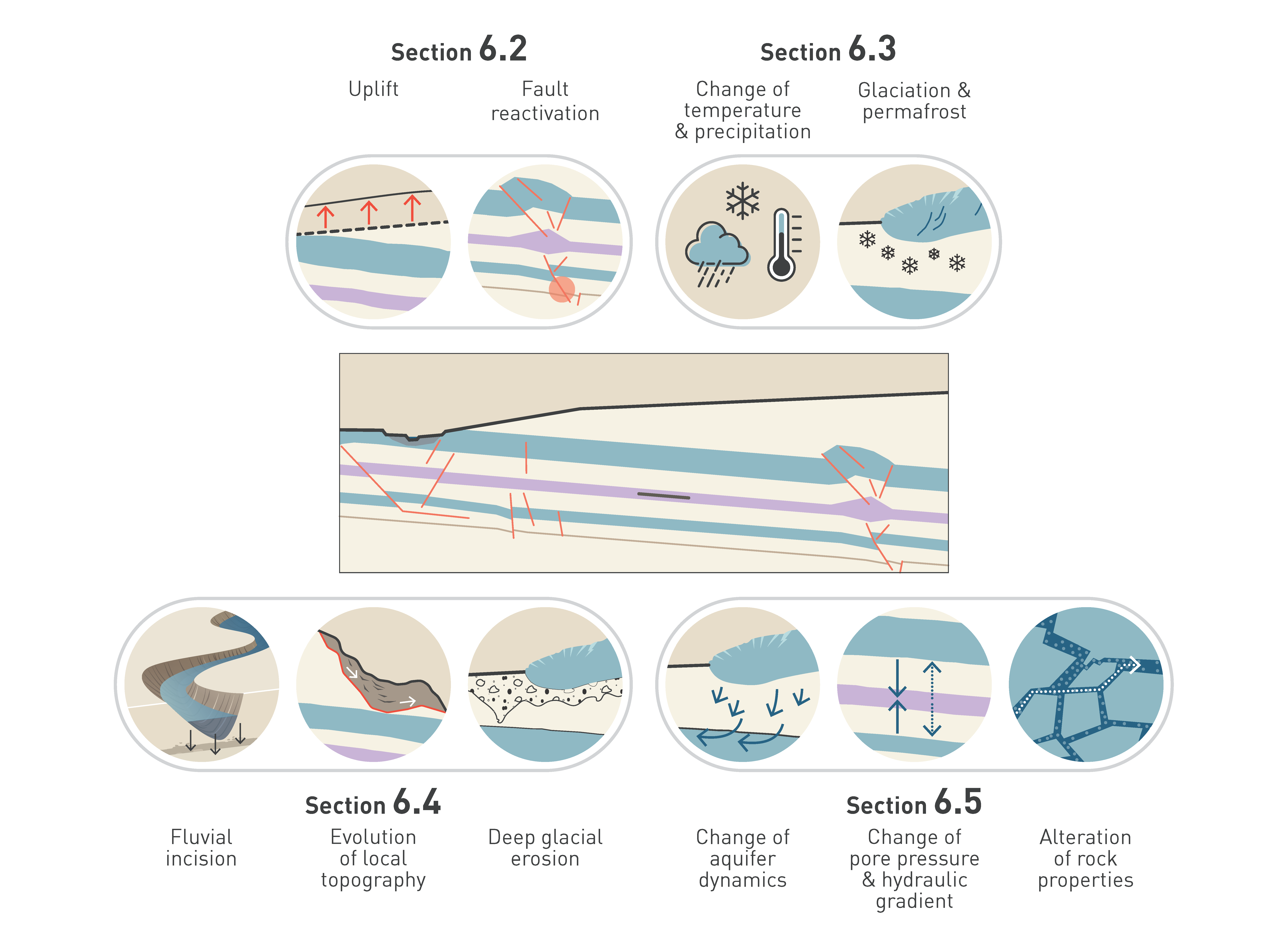
Fig. 6‑1:Schematic visualisation of the principal geological processes potentially affecting the geological barrier and corresponding structure of the chapter

The main aspects that are addressed with respect to future repository performance and long-term safety are tectonic evolution with vertical motion as a driver of erosion and fault reactivation potential (Section 6.2); climate evolution as a driver of erosion and changes in hydrogeological conditions, such as changes in temperature and precipitation as well as ensuing glaciations and the formation of deep-reaching permafrost (Section 6.3); erosion with the three main components fluvial incision, evolution of local topography, and deep glacial erosion (Section 6.4); and the hydrogeological evolution including changes in properties of the aquifer flow system and pore pressure and thus in the flow system and the alteration of porewater and dissolution processes (Section 6.5).

Given the known process rates and the geological and geomorphological characteristics of the siting regions, it is expected that future tectonic and climatic forcing will drive fault movement and surface processes (Fig. 6‑2) in Northern Switzerland, and the potential impact of these must be accounted for. This section provides an overview of the relevant processes, process inter­actions, and feedback to be expected in Northern Switzerland.

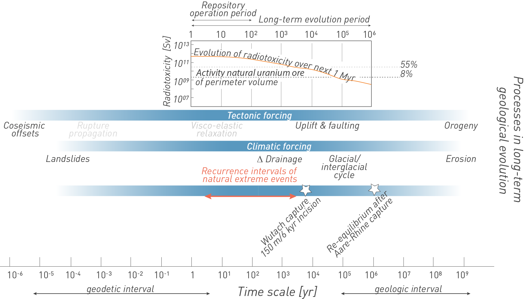
Fig. 6‑2:Geological processes acting at different timescales compared with the time period relevant for repository safety

The geology and geomorphology in the vicinity of the repository are expected to be subjected to tectonic and climatic forcing that drive erosional processes or fault motion that could potentially affect the stability of the geological barrier. Given the period under consideration of one million years for HLW (see figure above), several of these processes need to be addressed. Note the log-scale for the time of observation. Radiotoxicity is based on the Swiss waste inventory and is a measure that allows the comparison between radioactive waste and natural rock compositions, such as U-rich (Cigar Lake [8%], La Creusaz [55%]) rock types, assuming a similar volume as the HLW waste in their perimeter of tunnels and caverns (see Nagra 2024d). Also indicated are two examples of geomorphic events that have influenced the process rates in Northern Switzerland on different timescales: the capture of the Wutach River resulted in strong incision of which the majority of up to 150 m may have occurred during the first approximately six thousand years after the capture (Einsele & Ricken 1995). The reorganisation of the Aare – Rhine Rivers impacted Northern Switzerland regionally. Re-equilibrium of the drainage system to a capture ~ 4.2 Ma ago was modelled to take approximately one million years.

Tectonic and climatic drivers act on a variety of timescales (Fig. 6‑2), with short timescale events such as earthquakes or extreme climate-driven meteorological events, whether instrumentally or historically recorded, rarely being a good proxy for long-term behaviour. Conversely, studies that focus solely on geological archives and landforms on scales of 10⁵ to 10⁶ yr are often not precise enough to resolve discrete fault behaviour or to decipher the landscape response to climatic forcing. Therefore, earthquake and climate impact studies need to be integrated across multiple timescales, and observations extended to longer timescales spanning several thousand years to one million years to account for the potential future behaviour of different forcing factors that could reduce the efficiency of the geological barrier.

Consequently, any changes in topography and relief due to vertical crustal movements and super­imposed climate-driven changes in a tectonically active region will influence the form and rate of erosion processes. Thus, tectonic and climate-driven processes need to be identified, classified, and rated with respect to their relevance, timing, location, and potential impact on the geological barrier function. In the light of these considerations, the specific forcing factors that have determined, and will continue to influence, the long-term geological evolution of Northern Switzerland involve low-strain tectonic processes, climate change, and protracted erosion (see Fig. 6‑1). Taken together, these three components may influence the hydrogeology and geo­chemistry of the host rock and confining units, as explained below:

Tectonic evolution based on the present-day geodynamic configuration of the Alpine realm is expected to influence vertical and horizontal motion in the region. On a large scale, tectonic processes such as rock uplift of the Alpine Foreland and subsidence of the southern Upper Rhine Graben play an important role as they build topography and drive fluvial incision and denudation. Because the resulting erosion reduces the overburden thickness above the repository, the rates and patterns of such regional vertical motion have been assessed (see Section 6.2). Large-scale geodynamic processes, on geological timescales of millions of years (Chapter 3, Section 4.3), determine the orientation and magnitude of the regional tectonic stress regime, which might be altered on much shorter timescales by transient perturbations. These perturbations may, for instance, involve either lithospheric flexure because of regional loading and unloading during glacial advances and retreat or hydro-isostasy. Such processes can affect the aquifer flow system or hydraulic gradients (see Section 6.5), but they may also unclamp locked faults through the erosional reduction of normal stresses and trigger earthquakes with very long recurrence intervals (see Section 6.2.3).

Northern Switzerland is adjacent to a region where mantle-driven processes are responsible for magmatic activity and associated processes. Two of the closest centres of volcanic activity to Northern Switzerland are the Kaiserstuhl and Hegau Graben eruption centres in southern Germany. Volcanism at the Kaiserstuhl eruption centre occurred between ~ 21 and 13 million years ago, while volcanic activity in the neighbouring Hegau region ceased in the Late Miocene (Geyer et al. 2023). There has been no magmatic activity in Northern Switzerland for at least the last 5 million years (Schreiner 1992, Ibele 2015). Considering the current characteristics of the region, there are no indicators for dormant volcanic activity in Northern Switzerland, in contrast e.g. to the Eifel region in Germany. Seismicity in Northern Switzerland reflects low-rate tectonism (Diehl et al. 2023) with no documented volcanic tremors. Thus, volcanism in Northern Switzerland is considered very unlikely within the next one million years and is therefore of no concern and is not considered further here.

A characterisation of expected seismic or aseismic fault slip (see Section 6.2.3) is important to assess hydraulic changes and potential flow along faults in the low-permeability sequence. No relevant effects of seismic shaking on the integrity of the deep geological repository are expected because of the deep subsurface repository position and backfill (see Nagra 2024i). Seismic hazard during the operational phase is taken into account in the operational safety report (see Nagra 2024h and Nagra 2024g).

In this chapter, information is provided to answer the following questions:

• What uplift rates can be expected in the siting regions over the next 100'000 to one million years?

• What vertical motion is expected downstream and upstream of the siting regions along the main rivers, which may in turn influence future river incision?

• Where and to what extent is movement along faults possible?

Climate evolution in the northern sector of the Alpine region is expected to be influenced by recurring and protracted changes in the Earth’s orbit and tilt, which has had a major influence on landscape evolution during Pleistocene glacial/interglacial cycles. Because of the recurrent nature of these forcing mechanisms, they are expected to continue to exert this influence in the future. In particular, the change from a predominant ~ 41-kyr cycle to the establishment of a 100-kyr-long cycle during the Mid-Pleistocene Transition (MPT) fundamentally impacted erosional and sedimentary processes and thus Quaternary landscape evolution in Northern Switzerland (see Section 6.4.1). This cyclicity modulates climate parameters such as temperature and precipitation, which in turn influence water and sediment discharge as well as the overall hydrogeological evolution in the subsurface.

The greatest past climate impact on the landscape was associated with Pleistocene glacial periods (see Section 6.3). Extensive foreland glaciations can change sediment routing, deposition and drainage pathways or erode overdeepened valleys. In Northern Switzerland, it is expected that long durations of extensive foreland glaciations can, for example, cause lithospheric depression in the North Alpine Foreland along with transient stress changes that could influence the seismogenic behaviour of inherited faults (see Section 6.2.4). Typically, postglacial rebound follows an exponential trend until isostatic equilibrium is restored. During this period, higher uplift rates and associated stronger fluvial incision can be expected (see Section 6.4.3.1). In addition, mechanical loading and compaction by the ice cover, as well as subglacial infiltration, are likely to impact the hydraulic system. Extensive foreland glaciations may be accompanied by deep-reaching permafrost, which might affect aquifers by groundwater freezing and increase hydraulic heads and/or change groundwater flow paths (see Section 6.5.1.3).

Questions to be answered with respect to climate forcing are:

• What timing and extent of future glaciations in Northern Switzerland might be expected, considering natural conditions and potential effects of anthropogenic CO₂ emissions?

• What ice thicknesses and duration of ice occupation are expected during future glaciations considering Pleistocene examples?

• To what depth could the subsurface be frozen during future ice ages (permafrost)?

Erosion is mainly driven by the effects of tectonic and climatic processes, as outlined above and illustrated in Fig. 6‑2. In the area of the selected repository siting regions in Northern Switzerland, these processes may be characterised by slow vertical tectonic movements and glacial influences. The latter may involve significant erosional lag times between ice loading, topographic change, and deglaciation, as well as rate changes during isostatic readjustments. Ultimately, it is the synergistic interaction between long-term tectonic processes that build topography on the one hand and superimposed surface processes that are influenced by climate and vegetation cover on the other that sculpt landscapes (e.g. Burbank & Anderson 2012). The landscape of the three siting regions in Northern Switzerland has been primarily shaped by the stepwise fluvial incision of the Aare and Rhine Rivers, the evolution of a low-relief cuesta landscape, and repeated deep glacial erosion and depositional processes determined by the glaciations of the Alpine Foreland. Accordingly, the main drivers for these processes are the effects of glacial/interglacial cycles and long-term rock uplift associated with the vertical motion of the Alpine orogen and its foreland. However, the process rates are low in a global context and compared to seismically active plate-boundary settings.

To assess erosion with respect to the performance and long-term safety of the future repository, the following questions will be answered:

• To what extent will the overburden thickness be reduced at the repository sites? The answer to this question needs the following sub-questions to be addressed:

  • How will the fluvial system evolve? How much incision is expected during the period under consideration? Will the host rock and confining units remain below the local base­level?

  • How will the morphology around the repository evolve with regard to recharge and dis­charge areas?

  • How deep could future glacial erosion reach at the location of the future repository?

The cascade of driving forces outlined above leads to changes in the future landscape that also affect the hydrogeology and hydrochemistry in the rock column. Hydrogeological changes in areas subjected to multiple glaciations and tectonic uplift can be significant and the effects on the stability of the geological barrier are thus analysed in this regard. In hydrogeological systems, a geological barrier is typically subdivided into the host rock, the low-permeability confining units, and the surrounding deep aquifer systems. Not only do tectonic movements, climate change, and climate-driven surface processes (erosion) affect the recharge and discharge paths and gradients in deep aquifer systems, they can also impact the gradients in the low-permeability units. As a result of its high clay-mineral content (self-sealing capacity; Section 5.7) and low permeability (Section 5.6), there tends to be little impact of tectonics or erosion on transport in the Opalinus Clay. However, if overburden thickness decreases drastically because of erosion, decompaction effects may lead to less efficient self-sealing (Section 5.7), increased porosity and permeability (Section 5.6), and a change in host rock mineralogy and porewater chemistry.

The following main questions concerning the influences of tectonics, climate and erosion on the hydrogeology and barrier performance and thus the long-term safety of the future repository will be addressed:

• How could the dynamics in the deep aquifers evolve (flow velocity, flow direction, discharge paths)?

• Are the gradients across and along the low-permeability sequence (host rock and confining units) expected to change in a relevant way?

• What are the expected effects of the possible fault-slip scenarios?

• Will transport across the low-permeability units remain diffusion-dominated? Do diffusion and sorption properties change in a significant way?

• How might the porewater composition change in future and how might this impact diffusion and sorption of radionuclides?

Future tectonic activity in Northern Switzerland may affect the geological barrier properties of the host rock in the siting regions in two ways: (1) Rock uplift may increase topographic gradients and thus the potential for intensified erosion. (2) Seismic and aseismic fault slip may change the hydraulic properties along faults and thus the dominant transport mechanism. Consequently, both aspects need to be addressed and evaluated in detail.

This section summarises the knowledge on regional and local tectonic processes in Northern Switzerland. It builds on the geological evolution highlighted in Chapter 3 and provides additional detail about the present-day geodynamic context of Central Europe. Throughout the section, the term neotectonics is used to address seismogenic and aseismic deformation processes that have been active from Neogene times until the present day. This time period reflects the duration of the current stress regime, established since the last major tectonic reorganisation. In Northern Switzerland, this encompasses the period from the NW propagation of the Alpine deformation front (Early Miocene) and recorded décollement-related deformation in the eastern Jura Fold-and-Thrust Belt (Middle Miocene) until the present day (Section 4.3.5). The addressed period also includes the time of so-called active tectonics, i.e. as relevant for society (Wallace 1984, Nagra 2024l for more detail).

Section 6.2.1 starts with an overview of driving forces for neotectonic deformation within the European geodynamic framework. Seismicity, recent geodetic velocities, and the location of areas with potentially active tectonics in Northern Switzerland are introduced. This is followed by a brief outline of far-field tectonic drivers for the main erosion patterns and magnitudes that influence the siting regions (Section 6.2.2).

The focus of Section 6.2.3 is on regional neotectonic processes and rates in Northern Switzerland. Based on this, Section 6.2.4 discusses the future tectonic evolution and highlights the importance of reactivation of inherited faults, rather than formation of new faults. The main conclusions are summarised in Section 6.2.5. A more in-depth discussion of neotectonic observations is provided in Nagra (2024l).

Overall, the geodynamic setting of Central Europe (Fig. 6‑3a) is influenced by the convergence between the African and Eurasian plates (Chapter 3, Fig. 3‑12). The largest geodetic velocities and highest strain rates are measured in the eastern part of the African – Eurasian plate boundary zone in Greece and Turkey (e.g. DeMets et al. 1990, Serpelloni et al. 2022). Rates decline significantly towards the western plate boundary zones, closer to the Alps. The highest rates of deformation within the western plate boundary zone have been recorded along wide, diffuse deformation zones, such as the Apennines, the Dinarides, or the Betic Cordillera (see Fig. 6‑3a, b and c). Here, active deformation appears to be mainly influenced by independent microplate motion, such as the counterclockwise rotation of the Adriatic plate and Tyrrhenian and Aegean back-arc extension (e.g. Nocquet & Calais 2004, Piña‐Valdés et al. 2022; see Fig. 6‑3b for low geodetic rates, Fig. 6‑3c for diffuse seismicity and Fig. 6‑3d for S_Hmax indicators of stress regimes).

In the Alpine region, horizontal geodetic velocities are influenced by microplate deformation, but the rates are significantly lower and seismicity relatively sparse compared to the above-mentioned zones, despite considerable topographic relief and evidence for vertical motion (Fig. 6‑3a, b, c, Fig. 6‑4). Across the central Alps, shortening is low with values similar to the uncertainty (Sánchez et al. 2018).

Based on the global navigation satellite system (GNSS) measurements, the vertical velocity field of the Alps is in the order of ~ 2 mm/yr along the northward-convex border (Fig. 6‑4), increasing towards the central Alps and characterised by a generally positive correlation with topography (Sánchez et al. 2018, Piña‐Valdés et al. 2022, Serpelloni et al. 2022, Pintori et al. 2022). Total decadal-scale uplift is generally higher in the areas that undergo less horizontal shortening and, as such, is higher in the western and central Alps compared to the eastern part (Sternai et al. 2019). A tectonic contribution to rock uplift and exhumation appears to be pronounced in the eastern Southern Alps, where ~ 2 mm/yr movement between the Adriatic plate and stable Europe are accommodated (Sánchez et al. 2018, Sternai et al. 2019, Serpelloni et al. 2022). In addition to tectonic drivers, buoyancy forces associated with isostasy make a significant contribution to uplift (e.g. Sternai et al. 2019, Piña‐Valdés et al. 2022). Isostatically driven processes, such as postglacial or erosional rebound/unloading, slab detachment, as well as the effects exerted by the formation of dynamic topography (upper mantle processes) and the establishment of horizontal gradients associated with gravitational potential energy are considered to play a role (Sternai et al. 2019). Isostatic adjustment in response to deglaciation or erosion might cause uplift and can be in the order of 10 – 30% and 10 – 20% in the western and central Alps and up to 50% and 30 – 40% in the eastern Alps, respectively.

Towards the northern and southern Alpine Forelands, vertical velocities decrease to positive sub-millimetre and even to stable, zero mm/yr rates (Sánchez et al. 2018, Henrion et al. 2020, Pintori et al. 2022; Fig. 6‑4c). Low vertical velocities are observed in the Jura Mountains and the Molasse Basin (Fig. 6‑4c).

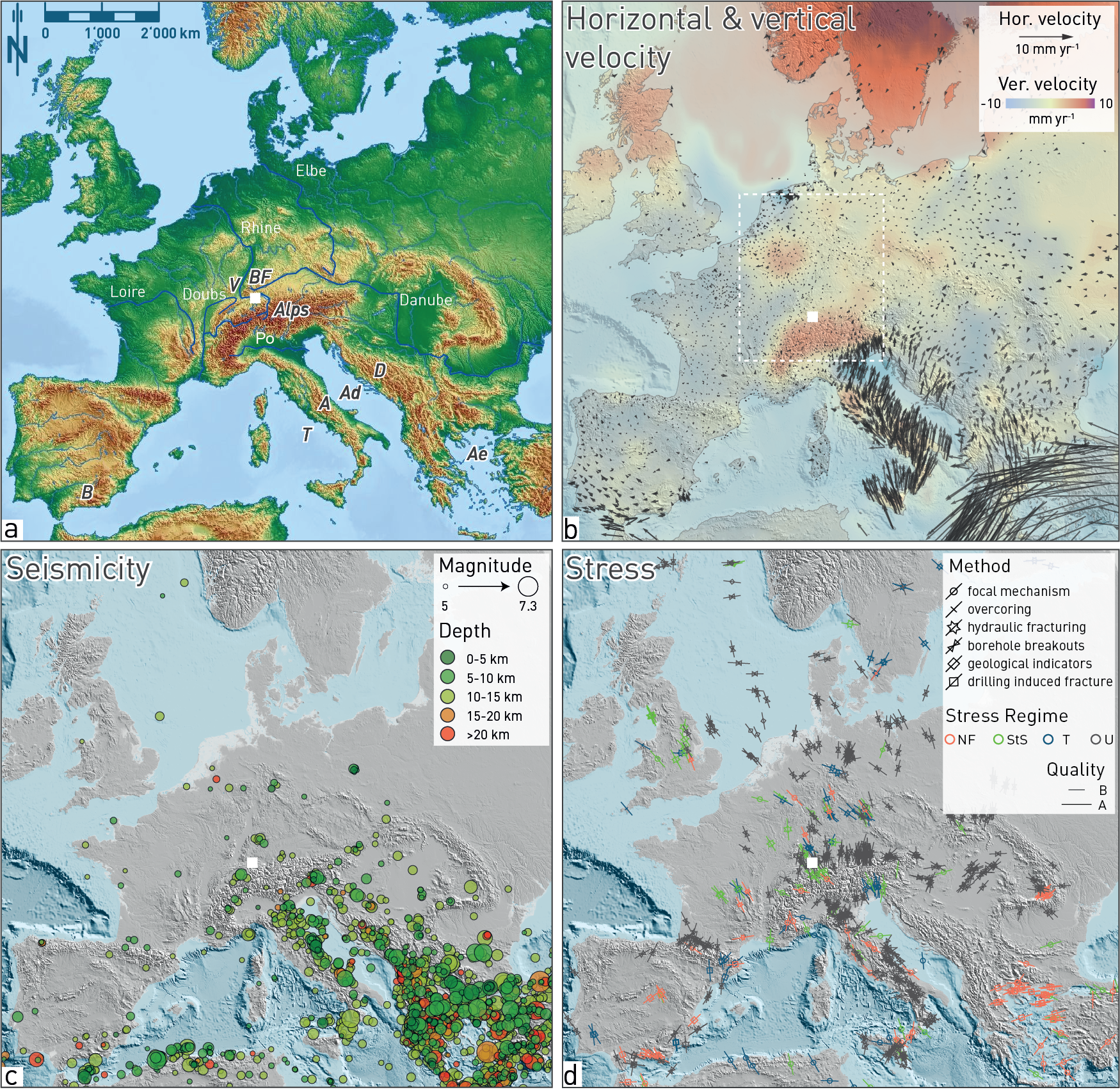
Fig. 6‑3:Velocity fields, seismicity and stress vectors in Europe

(a) Hillshade and digital elevation map of the same area with labels of geographic features discussed in Section 6.2.1. V: Vosges, BF: Black Forest, A: Apennines, B: Betic Cordillera, D: Dinarides, Ad: Adriatic Ocean, T: Tyrrhenian Ocean, Ae: Aegean. (b) By combining and harmonising geodetic velocities of several European datasets, a smoothed 3D velocity field solution across Europe and with respect to a stable Europe framework was generated (Piña‐Valdés et al. 2022). Dashed white rectangle outlines Fig. 6‑4. (c) Earthquakes with magni­tudes equal to and larger than 5 between 1900 and July 2023, colour-coded by depth (https://earthquake.usgs.gov/earthquakes/search/; retrieved July 10^th 2023). High-seismicity regions in Europe (e.g. Greece and Italy) are associated with subduction processes and coincide with regions of large horizontal velocities. (d) Direction of maximum horizontal stress and stress regime (Section 4.4). The map is based on the World Stress Map project (CASMO) and shows data from focal mechanism solutions, borehole breakouts, hydro­fractures etc. Stress indicators are colour-coded by their respective stress regime (Heidbach et al. 2016, 2018). NF: Normal fault, StS: Strike-slip fault, T: Thrust, U: Unknown. White solid square in all figures depicts the study area.

In this section, the regional geodynamic setting is reviewed with respect to its influence on erosion processes. Beyond the North Alpine Foreland, this primarily considers fluvial incision by the Rhine River system from source to sink. Here, it is considered how rates of deformation (mainly vertical motion) have driven baselevel changes of the Rhine on timescales similar to the future one million years. This information is important to assess future fluvial incision, as rock uplift is expected to exert a first-order control.

The Aare – Rhine River system hydrologically connects the Alps with the North Sea as the final baselevel (Fig. 6‑4a). From source-to-sink, the Rhine crosses several tectonic domains that may influence erosion (Fig. 6‑4b and Fig. 6‑5). The siting regions are located along the Hochrhein section, between the Bodensee and Upper Rhine Graben (Fig. 6‑4a).

The main neotectonic influence on erosion in Northern Switzerland are Alpine uplift, trans­tensional deformation in the Upper Rhine Graben and potential low-level movements of the Jura Fold-and-Thrust Belt and the Bodensee – Hegau Graben (see Section 6.2.3). Together these define the regional tectonic setting for fluvial erosion processes associated with rock uplift and baselevel drop.

Fluvial incision and erosion in Northern Switzerland are also influenced by far-field uplift of the Eifel area and the Rhenish Massif (Fig. 6‑3b, Fig. 6‑4, Fig. 6‑5). The latter represents a regional intermediate baselevel of the Rhine. As long as the area continues uplifting, it is not expected that processes related to sea level changes will affect the siting regions on the relevant timescale of one million years. The main tectonic domains that are located between the Rhenish Massif and the Alpine Foreland, which control stream profile evolution of the Rhine River, are summarised below, starting at the relevant downstream locations (see Nagra 2024k for more detail).

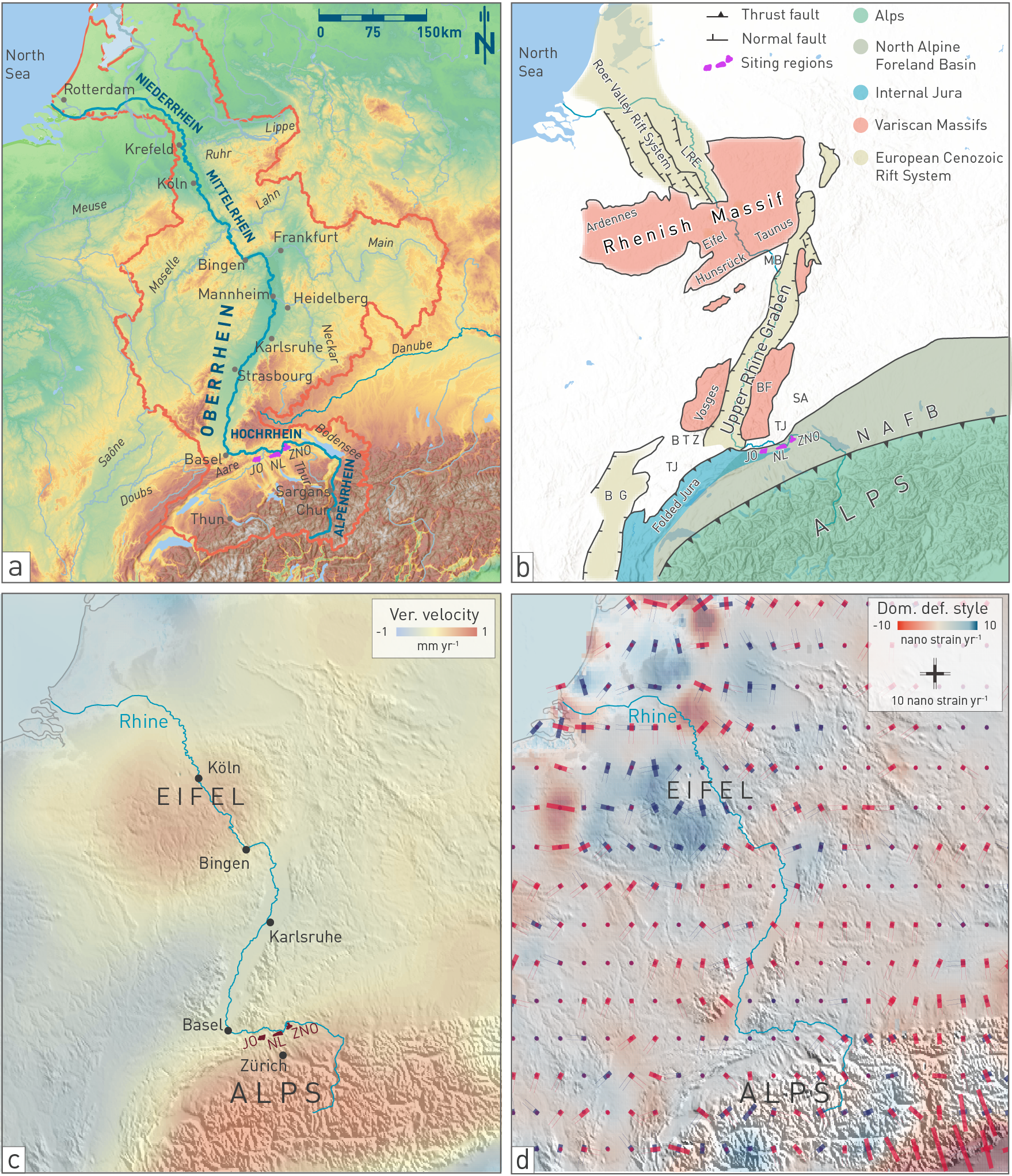
Fig. 6‑4:Present-day Rhine catchment in a morphotectonic and geodynamic context for fluvial incision and sediment accumulation

(a) Rhine catchment (b) Morphotectonic domains. The course of the Rhine River is highlighted with dark blue line. BF: Black Forest, BG: Bresse Graben, BTZ: Bresse Transfer Zone, TJ: Tabular Jura, LRE: Lower Rhine Embayment, MB: Mainz Basin, NAFB: North Alpine Foreland basin, SA: Swabian Alb. Data source: EU-DEM (European Environment Agency), rivers based on European Environment Agency (2020), https://land.copernicus.eu/en/products/eu-hydro/eu-hydro-river-network-database. c) Geo­detic velocities (redrawn from Piña‐Valdés et al. 2022). Vertical motion relative to stable Europe is highlighted by red and blue colours (uplift and subsidence, respectively). The Alps and the Eifel area are prominent uplift regions that influence the profile of the Rhine River. (d) Strain rates (redrawn from Piña‐Valdés et al. 2022) with red pins showing contraction and blue pins showing extension) are generally low within the Alpine Foreland.

Rhenish Massif, Upper Rhine Graben and Vosges and Black Forest Massifs

The Rhenish Massif represents an actively uplifting region, which is coincident with bedrock incision of the Rhine River (Mittelrhein, see Fig. 6‑4 and Fig. 6‑5). It has been uplifting since at least Oligocene times (Illies & Greiner 1979, Illies et al. 1979, Garcia-Castellanos et al. 2000, Ziegler & Dèzes 2005, 2007). Extensive volcanism in the area, spanning from the Oligocene (Westerwald) until the Late Quaternary (East and West Eifel; Schmincke 2007), is closely connected with asthenospheric upwelling associated with a plume (Ritter & Christensen 2007). Staircase river terraces document incision that has apparently accelerated since the Pliocene (Fuchs et al. 1983) or the latest Early to Middle Pleistocene (Meyer & Stets 1998), with the greatest amount of incision (up to 250 m) achieved during the past 880 kyr. While the afore­mentioned authors interpret the incision to be a response to uplift only, Demoulin & Hallot (2009) suggest that part of the total incision might be related to knickpoint retreat in tributaries rather than tectonic deformation. If correct, this process may reduce the total uplift to 140 m, yielding a Quaternary long-term uplift rate (since ~ 880 ka) of ~ 0.2 mm/yr (Demoulin & Hallot 2009). GNSS data of the Eifel area indicate an overall present-day uplift in the order of 0.5 – 1 mm/yr (Fig. 6‑4c), which is likely related to mantle activity (Piña‐Valdés et al. 2022, Henrion et al. 2020). Combined, these data suggest long-term and ongoing uplift of the Rhenish Massif – Eifel area at amounts that exceed eustatic sea-level changes. It is reasonable to assume that these processes will continue in the future. Under this assumption, the Mittelrhein section (Fig. 6‑4a) would constitute an intermediate baselevel for the longitudinal profile of the Rhine.

The Upper Rhine Graben is part of the European Cenozoic Rift System (ECRIS). It is bordered to the northwest by the uplifting Rhenish Massif, to the south by the Jura Fold-and-Thrust-Belt, by the Vosges Mountains in the west and the Black Forest in the east (Fig. 6‑4 and Fig. 6‑5). Here, the Rhine (Oberrhein) drains a tectonic domain characterised by long-term intermittent sub­sidence, accompanied by erosion of the uplifting rift shoulders.

The present-day depositional centres (the northern, very deep Heidelberg Basin and the southern, less deep Geisswasser Basin) were established at least during the Pliocene – Quaternary. At this time, the central part of the Upper Rhine Graben was located in a restraining bend (Schumacher 2002) explaining the low subsidence and low sedimentation observed in this area (Karlsruher Swell; e.g. Gabriel et al. 2013, Edel et al. 2007, Hagedorn & Boenigk 2008, Rotstein & Schaming 2011). Importantly, the contrasting subsidence rates between Karlsruher Swell and Geisswasser Basin are expected to flatten the Oberrhein profile, leading to further deposition upstream. The Karlsruher Swell thus represents a buffer against increased incision. Quaternary subsidence rates are in the order of 0.1 – 0.3 mm/yr, increasing substantially towards the northern Upper Rhine Graben (Berger et al. 2005, Hagedorn & Boenigk 2008, Peters & van Balen 2007, Preusser et al. 2021).

Based on precise levelling data, Fuhrmann et al. (2014) inferred that the Upper Rhine Graben is mainly subsiding at rates between ‑0.2 and -0.5 mm/yr, which they attributed mainly to a combination of tectonic subsidence and sedimentary load (e.g. compaction and isostatic effects). This pattern is contemporaneous to slight uplift of up to 0.3 mm/yr of the graben shoulders at Black Forest and Vosges Massifs (relative to a reference point at the location of Freudenstadt in the eastern Black Forest Massif).

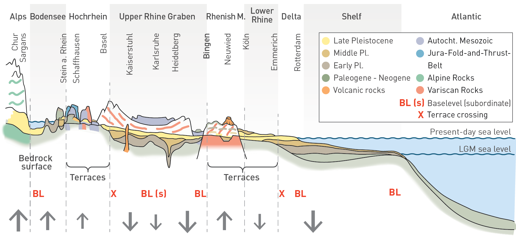
Fig. 6‑5:Sketch of the Rhine River course with domains of Quaternary vertical motion

Schematic river course with simplified general geology, occurrence of fluvial terraces and location of terrace crossings, (intermediate) baselevels of regional relevance, and variability of sea level. Not to scale, after Neeb in Hinderer (2005) and Hinderer (2012). Tectonically driven rock uplift and basin subsidence (qualitatively marked by the grey arrows) influence the pattern and rates of fluvial incision along the Rhine. Northern Switzerland is mainly influenced by North Alpine Foreland rock uplift, subsidence of the Upper Rhine Graben, and rock uplift of the Rhenish Massif. Figure draft courtesy of H.A. Kemna.

North Alpine Foreland

The dominance of Alpine-related uplift (including tectonic and isostasy-driven processes) within the North Alpine Foreland results in a general surface uplift gradient oriented perpendicular to the Alpine front with rates that decline towards NNW (Fig. 6‑6; Champagnac et al. 2009, Mey et al. 2016). This trend is also revealed by long-term thermochronology data (Fox et al. 2016), basin-wide erosion rates (Wittmann et al. 2007, Delunel et al. 2020) and measurements of present-day vertical motion (GNSS, precise levelling, e.g. Schlatter 2013, Nagra 2024l). The roughly north-south trend is also reflected by the principal flow direction of the larger rivers traversing Northern Switzerland, which suggests a long-term tectonic control on the geomorphic characteristics of this region.

Northern Switzerland is influenced by glacial/interglacial cycles with growth and decay of the Alpine Ice Field, including a number of large foreland glaciations (Section 3.5, Section 6.3; Nagra 2024j). Accordingly, Northern Switzerland is expected to undergo glacial isostatic adjustment (GIA), which affects the temporal and spatial uplift distribution (e.g. Craig et al. 2016). From studies related to large continental ice shields, it is known that GIA-related uplift after the Last Glacial Maximum (LGM) deglaciation shows a quasi-exponential form with fast and high-rate uplift shortly after deglaciation and continuously decreasing rates (see for instance Turcotte & Schubert 2014). A GIA effect might be still detectable in the Alpine Foreland, albeit to a lesser extent than in the Alps or in areas of large continental ice shields because of thinner ice and shorter duration of glaciation (see Section 6.3.2 and Nagra 2024j).

Long-term uplift proxies in Northern Switzerland (based on exhumation and incision rates)

Using exhumation or fluvial incision rates as proxy for rock uplift (which is the most important input parameter for the assessment of future erosion) is a simplification that requires the assump­tion of steady-state topography. Nevertheless, it allows a valuable first-order uplift estimate on long timescales, when short-term fluctuations level out. However, because of the complexities in tectonically active regions and the influence of climate fluctuations, this assumption needs to be treated with caution.

Past exhumation of the Molasse Basin is summarised in Section 4.3.5 and Chapter 3. Here the focus is on the second exhumation phase, which resulted in the present-day configuration. The amount of Miocene/Pliocene exhumation is generally estimated around 1 km (e.g. Mazurek et al. 2006, Villagómez Díaz et al. 2021, Omodeo-Salé et al. 2021, Schegg & Leu 1998). However, the timing of onset of exhumation is debated, with estimations ranging between 12 Ma and 5 Ma (von Hagke et al. 2015, Looser 2022, Mazurek et al. 2006, Villagómez Díaz et al. 2021). Under the simplest assumption of linear exhumation, inferred exhumation rates range between ~ 0.08 mm/yr and 0.20 mm/yr. However, it should be noted that several studies indicate heterogeneous exhu­mation rates in the past ~ 10 Myr.

Bedrock incision rates based on Quaternary geomorphic markers that are often used as proxy for rock uplift cannot be directly converted in Northern Switzerland. Here, effects of exhumation are complicated by the impact of baselevel lowering resulting from changes in drainage routing (see Sections 3.5 and 6.4.1.2). Nevertheless, a first-order assessment of bedrock incision can be calculated from bedrock elevation changes and the age of the Deckenschotter sediments (see Chapter 3 and Fig. 6‑6c to e). Mean ages of 1.38 ± 0.31 Ma and 0.9 ± 0.13 Ma were assumed for the Höhere Deckenschotter (HDS) and Tiefere Deckenschotter (TDS), respectively to derive the incision rates shown in Fig. 6‑6c to e (see Nagra 2024k for details on age determination). These rates (~ 0.1 – 0.2 mm/yr) are based on the elevation difference between the lowest data point of a respective Deckenschotter outcrop (Heuberger & Naef 2014) and the local erosion base (LEB). Incision rates increase slightly (mean rates HDS to LEB ~ 0.14 to 0.25 mm/yr and mean rates TDS to LEB ~ 0.2 to 0.32 mm/yr), if analysed along the valleys straddled by the Deckenschotter deposits and if using locally derived ages as well as the age ranges derived from samples across Northern Switzerland (see Nagra 2024k). Note that the incision signal not only includes a share from drainage reorganisation but is also a mixed signal stemming from rock uplift of the Alpine Foreland and baselevel fall at the transition to the Upper Rhine Graben. This may be seen in the the interpolated isolines of HDS to LEB and TDS to LEB heights (Fig. 6‑6c and d) that are slightly rotated to a more NW-SE trend compared to levelling data and GNSS measurements (Fig. 6‑6a and b).

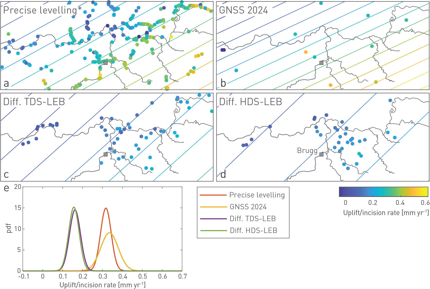
Fig. 6‑6:Patterns and rates of surface uplift and incision proxies on different timescales

The uplift planes in (a) to (d) are calculated from point measurements based on a regression using the coordinates as independent variables. (a) The interpolation of precise levelling data shows a gradient at an azimuth of ~ 153°, perpendicular to the Alpine front and declining towards the foreland. Vertical rates are measured with respect to Laufenburg. * 0.28 mm/yr were added to the dataset of precise levelling, which corresponds to the GNSS-based rate at which Laufenburg is currently uplifting with respect to stable Europe. (b) Interpolation of the vertical GNSS data shows a similar pattern to precise levelling data at an azimuth of ~ 157°. (c) Interpolation of height differences between the geomorphic marker represented by the local erosion base (LEB, see Section 6.4.2.1 for definition) and the base of the Tiefere Deckenschotter (TDS) using a mean age of 0.9 Myr. (d) Similar to (c) but using the Höhere Deckenschotter (HDS) as marker and a mean age of 1.38 Myr. See Section 6.4.1.2 for a discussion of the age constraints for the Deckenschotter deposits. Note that the elevation differences are based on the lowest elevation of each mapped Deckenschotter occurrence (Heuberger & Naef 2014). (e) Probability density function of all uplift proxy data shown in the respective maps above calculated as an example for the location of the city of Brugg (square in maps). Note the higher rates of present-day geodetic surface uplift signals with respect to the longer-term incision rates. LEB: Local erosion base.

Short-term geodetic surface uplift rates in Northern Switzerland

Present-day surface uplift rates as derived from geodetic measurements (precise levelling and GNSS) are considerably higher compared to past exhumation rates or incision rates using these as proxy for long-term surface uplift. However, present-day surface uplift rates for Northern Switzerland agree with each other, when accounting for the different reference frames (Fig. 6‑6a and b). The study area is currently uplifting at rates between ~ 0.2 and 0.5 mm/yr (Fig. 6‑6 and Fig. 6‑7). More detailed analyses are reported in Nagra (2024l).

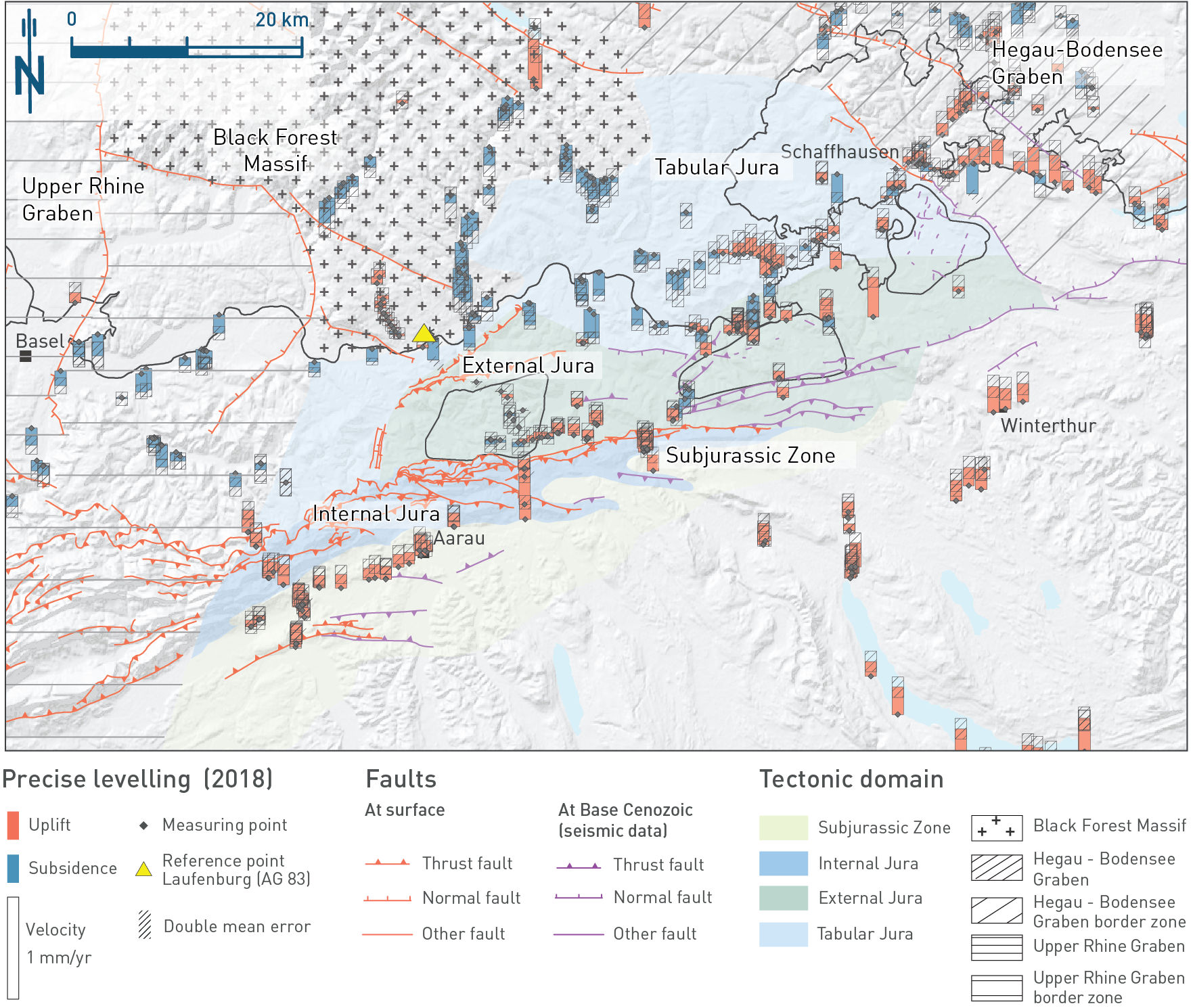
Fig. 6‑7:Geodetic precise levelling data with measurement uncertainties

Precise levelling measurements (analysis NEOTEK2018 by swisstopo). Only data with a good geological quality ranking (> 8.5) are shown. Vertical velocities are based on levelling measurements relative to the fixpoint Laufenburg (yellow triangle). These data show a general trend of decreasing rates from the Alps towards the foreland. Note that only a selection of the structures from 3D seismic interpretation is shown to highlight the structural trends of regional importance. These were projected from Top Villigen Formation to Base Cenozoic.

Summarising the domains crossed by the Rhine River, it can be concluded that the main influence on the incision of the Hochrhein are low rates of North Alpine Foreland rock uplift, compared with low, potentially episodic subsidence within the Upper Rhine Graben. The longitudinal Rhine River profile is also influenced by continuous uplift of the Rhenish Massif and Eifel areas. Accordingly, the Hochrhein is presently buffered against fluvial processes approximately down­stream of the city of Bingen (Fig. 6‑5).

All currently available data suggest that Northern Switzerland can be considered as an area characterised by low geodetic velocities. While the focus of the previous section was on vertical crustal motion (as a driver for erosion), this section highlights two additional datasets that provide evidence for ongoing tectonic activity in Northern Switzerland: (i) GNSS measurements at perma­nent stations, and (ii) the present-day earthquake distribution suggesting activity along major faults. The regions that record active deformation on multi-decadal timescales are the Upper Rhine Graben, the Hegau – Bodensee Graben and the Jura Fold-and-Thrust Belt.

Global navigation satellite system (GNSS)

Precise positioning measurements using permanently installed stations are used to monitor present-day motion (vertical and horizontal) at the Earth’s surface. Such a network of permanent stations also exists in Switzerland and has been densified in Northern Switzerland (Nagra 2024l). It is observed that, in particular in the early time after installation, the stations are characterised by higher velocities which are probably related to artefacts. Stations with longer monitoring periods show more stable velocity fields (Nagra 2024l). Generally, the resolution for horizontal motion is difficult to quantify, but inferred to be close to 0.1 mm/yr or below (e.g. Fig. 6‑8).

For a tectonic interpretation of the permanent stations located in Northern Switzerland, the hori­zontal motion is calculated in reference to stable Europe (Nagra 2024l). In general, horizontal velocity of the stations reveals a motion towards the NNE (Fig. 6‑8). No differential movements above the general noise level between neighbouring stations are detectable. Thus, no significant tectonic activity above the detection limit or referable to specific regional faults can be detected via GNSS. The data are thus averaged over the entire Northern Switzerland to constrain average velocity anticipated to occur in the future.

To do so, the horizontal velocity vector from each permanent station is subdivided into a north component and an east component (Fig. 6‑9). The east component is low, generally below 0.2 mm/yr for the considered stations. The north component is around 0.4 mm/yr. A slight decrease in the north component is observed in more northerly stationsFig. 6‑10. The weak linear regres­sion (Pearson’s r = -0.30) indicates 1.4 × 10^-9 ± 0.8 × 10^-9 yr^-1 shortening or 1.4 ± 0.8 m/km/Myr (Nagra 2024l). The shortening amounts to 2.8 × 10^-9 ± 0.9 × 10^-9 yr^-1 if only the stations around the siting regions, which were built with focus on detecting potential tectonic activity (red in Fig. 6‑9, Pearson’s r = -0.71), are considered. This estimate is subject to substantial uncertainties and thus only serves for an order of magnitude estimation. The inferred strain rate agrees well with published data for Northern Switzerland also based on GNSS movements and is indicative for low rates of horizontal motion for Northern Switzerland (Sánchez et al. 2018, Houlié et al. 2018, Rabin et al. 2018, Piña‐Valdés et al. 2022, Serpelloni et al. 2022). A very weak linear regression (Pearson’s r = 0.03) indicates 0.1 × 10^-9 ± 0.6 × 10^-9 yr^-1 E-W directed extension (Nagra 2024l). It should be noted that the E-W directed trend with respect to station position along strike of the Alpes is not statistically robust but serves as estimate of order of magnitude. All recorded rates using GNSS are significantly lower than the typical time-averaged bulk strain rates in an orogen of 3 × 10^-7 yr^-1 as proposed by Fagereng & Biggs (2019). Therefore, it is con­cluded that Northern Switzerland is currently deforming at low rates.

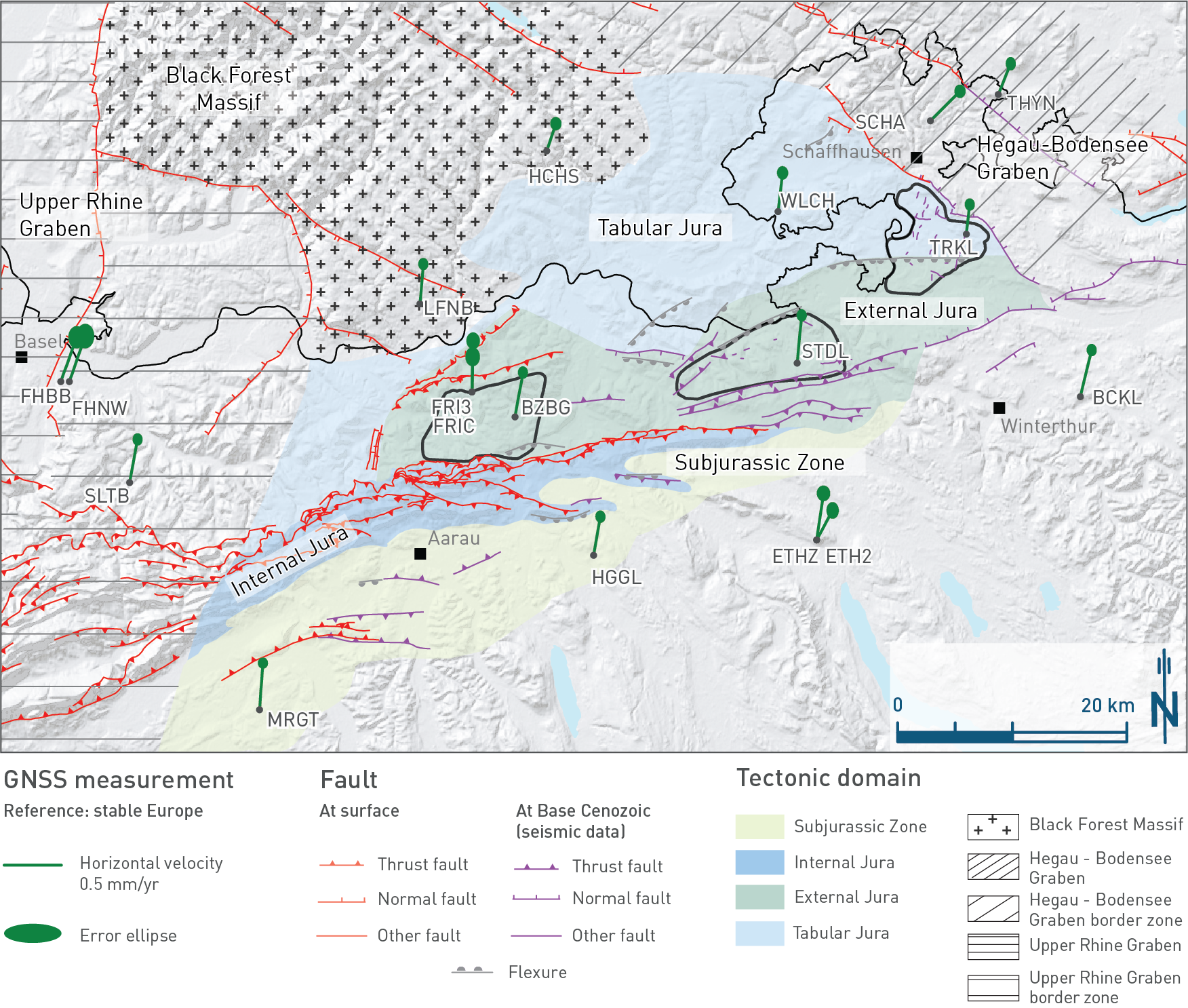
Fig. 6‑8:Present-day horizontal motion of permanent GNSS stations in Northern Switzerland

Results are calculated in reference to the ETRF 2014 (i.e. relative to stable Europe repre­senting a combination of the stations GRAS (Austria), JOZE (Poland), METS (Finland), ONSA (Sweden), POTS (Germany), WTZR (Germany), YEBE (Spain) and ZIMM (Switzer­land). Stations with two vectors (ETHZ, ETH2, FRI3, FRIC) have two antennas at close distance. Fault inventory shows traces of faults mapped at the surface (red) or on Base Cenozoic (violet). Note that only a selection of the structures from 3D seismic interpretation is shown to highlight the structural trends of regional importance. These were projected from Top Villigen Formation to Base Cenozoic.

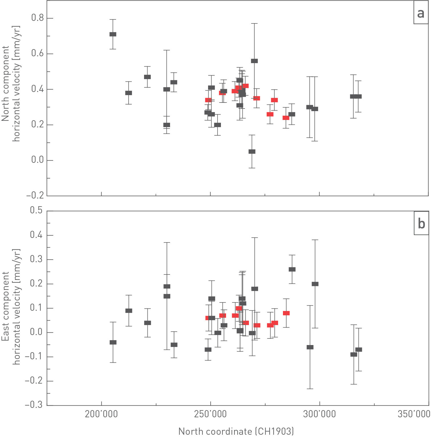
Fig. 6‑9:Horizontal velocity components deduced from repeated GNSS measurements

Stations are located over approximately 120 km north-south and 200 km east-west extent centred over Northern Switzerland. (a) North component of horizontal velocity vector plotted against the north coordinate of the station. (b) East component of horizontal velocity vector plotted against the north coordinate of the station. Results are in reference to the ETRF 2014 (i.e. relative to stable Europe representing a combination of the stations GRAS (Austria), JOZE (Poland), METS (Finland), ONSA (Sweden), POTS (Germany), WTZR (Germany), YEBE (Spain) and ZIMM (Switzerland)). Red-labelled stations are NaGNet stations, whereas black-labelled stations are AGNES stations (AGNES: Automated GNSS Network for Switzerland). Stations are shown in Fig. 6‑8. Stations with two vectors (ETHZ and ETH2, FRI3 and FRIC) have two antennas close-by.

Seismicity

Switzerland has a well-documented historical record of seismicity, which dates back several hundred years for felt seismicity (Fäh et al. 2011). The density of seismic stations was gradually increased over the past decades and now allows to determine earthquakes with magnitudes below 1.5 nearly everywhere in Switzerland and magnitudes even below 0.75 in the area comprising the siting regions (Nagra 2024l). Although earthquakes have been recorded in the area close to the siting regions, Northern Switzerland is one of the areas of lowest determined seismicity within the country (Fig. 6‑10).

The largest known historical earthquake in the vicinity of the siting regions, located at the overlap between the Jura Fold-and-Thrust Belt and the Upper Rhine Graben, is the M_w 6.6 Basel earth­quake in the year 1356 (Bakun & Scotti 2006, Fäh et al. 2011). Other historical and instrumentally recorded events had significantly smaller magnitudes (Fig. 6‑10). The spatial distribution of seismicity in Northern Switzerland can be loosely correlated with the occurrence of the large tectonic domains. For example, the area around Basel with a comparatively higher level of seismicity is located in the Upper Rhine Graben (Fig. 6‑10, see Section 4.3.3). Earthquakes in the Upper Rhine Graben have focal mechanisms typically indicating transtensional deformation (Fig. 6‑10). Similarly, the Hegau – Bodensee Graben, which extends from the Bodensee to the NW (see Section 4.3.3), is characterised by increased present-day seismicity (Kahneman et al. 1982). Focal mechanisms of a series of earthquakes occurring between 2014 and 2019 located along the Neuhausen Fault within the Hegau – Bodensee Graben are characterised by predominant normal faulting (Fig. 6‑10; see Diehl et al. 2023 and Nagra 2024l for more detail).

In the Jura Fold-and-Thrust Belt seismicity is concentrated in the central to western parts but is indicative of ongoing deformation in the Internal Jura (e.g. Lanza et al. 2022). Between these tectonic domains, seismicity in Northern Switzerland is sparse and earthquake hypocentres are distributed throughout the entire upper crust. A cluster of shallow, low-magnitude events occurs near the city of Eglisau (Fig. 6‑10; see Nagra 2024l).

Glacial isostatic adjustment is known to influence not only the vertical surface velocities but also the horizontal velocity field. These effects are not only seen in the immediate vicinity of the glacial load, but also at long distances away (e.g. Grollimund et al. 2001), hence phases of increased fault activity need to be considered in association with glacial cycles, especially for a prolonged period following deglaciation. While glacial isostatic adjustment can perturb the overall stress field and thus inhibit or trigger faulting (e.g. Hetzel & Hampel 2005, Craig et al. 2016), it is unlikely that glacial isostatic adjustment alone is responsible for fault failure especially at a distance from the ice load (Craig et al. 2023).

Taking these considerations into account, it can be concluded that the timing of seismicity in Northern Switzerland might be predominantly caused by transient non-tectonic stress per­turbations (e.g. related to glacial isostatic adjustment), while the overall mechanism of strain release follows the elastic long-term tectonic strain stored in the lithosphere. This tectonic strain is expected to be released along the pre-existing (regional) faults, as such faults have been repeatedly reactivated during the tectonic evolution (Section 4.3). In conclusion, Northern Switzerland is considered as tectonically active, but it is a low-strain area (see Nagra 2024l).

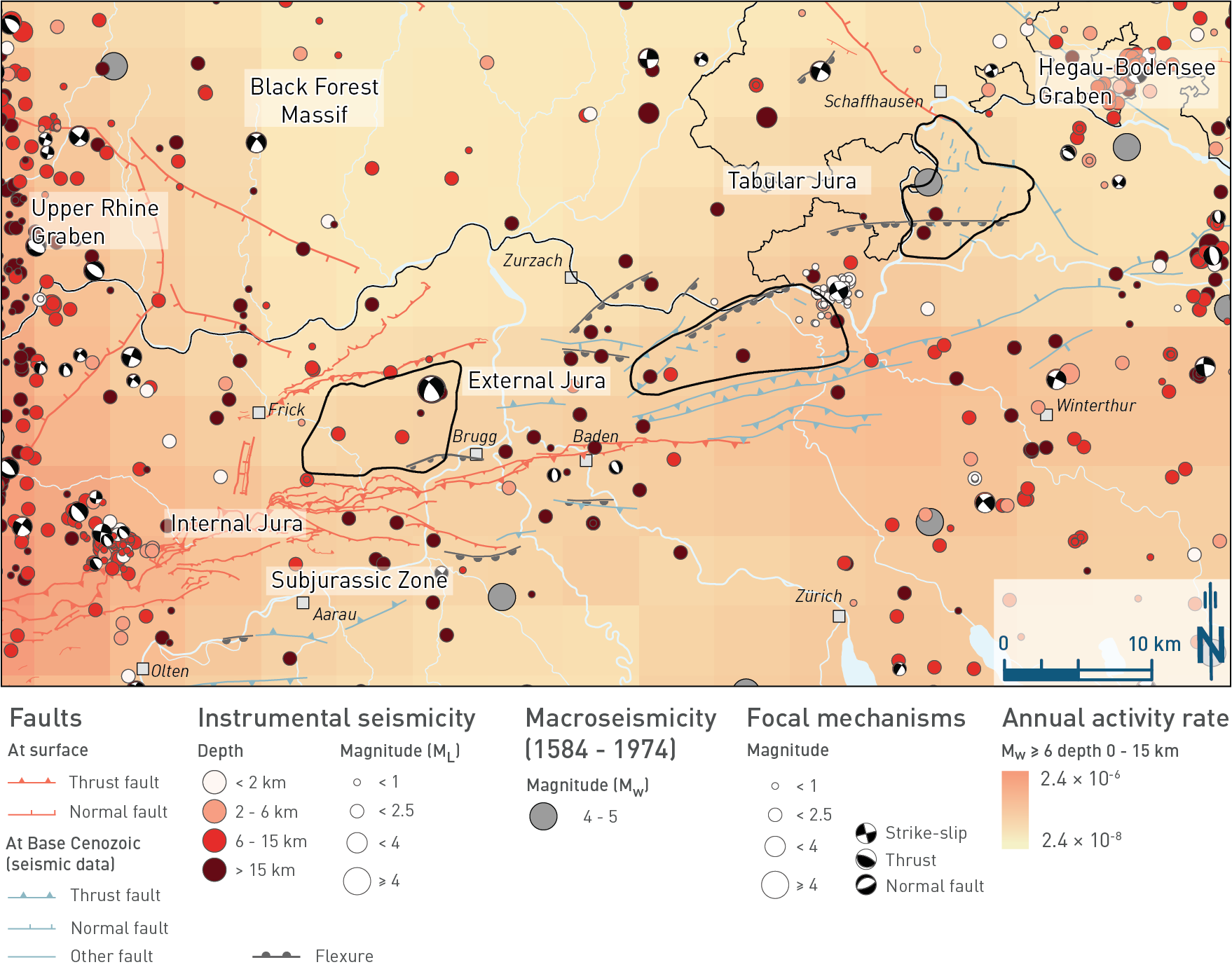
Fig. 6‑10:Distribution of earthquakes and selected focal mechanisms

Recorded earthquakes (historical and instrumental) and modelled probability of earthquakes with M_w ≥ 6 occurring in Switzerland, determined within the framework of the PRP project (swissnuclear 2013). The background colour indicates the annual probability of occurrence for earthquakes with M_w ≥ 6 in an area of 0.05° longitude × 0.05° latitude (ca. 21 km²) for hypocentral depths < 15 km. Seismicity is based on different catalogues: historical data prior to 1975 (Fäh et al. 2011) and instrumental data between 1975 and October 2023 (merged catalogue with data until 2023/10/03, including Swiss Instrumental Network, absolute re-localised events (following Diehl et al. 2021) and regional analyses of selected earthquake clusters; courtesy of T. Diehl). Focal mechanisms are shown for selected events of the instru­mental catalogue. Note that only a selection of the structures from 3D seismic interpretation is shown to highlight the structural trends of regional importance. These were projected from Top Villigen Formation to Base Cenozoic.

Tectonic deformation across Northern Switzerland is anticipated to continue at low rates in the future. The future evolution of Northern Switzerland with respect to tectonic loading is expected to be strongly controlled by the protracted effects of the Alpine orogeny, as the Swiss Molasse Basin and the Jura Fold-and-Thrust Belt are part of the North Alpine Foreland and form a mechanical wedge with the interior part of the Alps (Section 4.3).

With respect to the anticipated continued deformation in the siting regions three observations are particularly important:

(i) The past tectonic evolution reactivated inherited faults acting as zones of weakness within the less deformed rock volume (Section 4.3). It should be noted that the retrieved core material drilled within less deformed rock volume contains evidence for strain accumulation also in the rock volume in-between the regional fault zone. The accumulated strain is substantially lower than in the regional fault zones. This is exemplified in the small number of seismically mappable faults (Nagra 2024a, 2024b, 2024c). The phenomenon that inherited faults within the crust guide sub­sequent strain has been previously reported in literature (e.g. Cooke & Madden 2014, Bürgmann & Dresen 2008, Handy & Brun 2004, Cooke & Murphy 2004, Zoback et al. 2002, Townend & Zoback 2000, Kirby 1985).

(ii) The overall geometry of the regional fault zones inferred from seismic reflection data seems suitable for allowing future slip along the fault plane and thus dissipation of strain. Gently dipping fault segments are more prone to reactivation under thrusting, whereas steeper fault segments will preferentially accommodated strike-slip movements and normal faulting.

(iii) Strain rates inferred from the recent GNSS measurements are low. This implies that the anticipated total strain over the temporal and spatial scale considered for the deep geological repository is limited. Furthermore, the strain rates inferred from GNSS are comparable to strain rates inferred for the main folding and thrusting of the Jura Fold-and-Thrust Belt (Section 4.3.5).

Based on the aforementioned considerations, the most likely tectonic evolution for the next one million years is formulated with ongoing low-rate tectonic loading resulting in homogeneous N‑S shortening and subordinate E-W extension across the siting regions. In addition, ice (un)loading and erosion are likely to predominantly affect the vertical component of the stress tensor and thus potentially impact fault reactivation. The predominant part of the anticipated strain will be dissi­pated along inherited regional fault zones.

The rock volume in-between the regional fault zones is likely to experience very limited amounts of strain. The evidence for reactivation of inherited faults and the concentration of instrumentally recorded seismicity along such structures provides a strong argument for tectonic stability of the potential disposal zones (Nagra 2024l). Nevertheless, the growth of new faults cannot be entirely excluded, but corresponding fault length and offset will be limited (Nagra 2024i).

The overall Cenozoic tectonic evolution of Northern Switzerland is an important driver for erosion, while seismicity and faulting are important factors that may affect long-term barrier performance. With respect to the assessment of future tectonic evolution, it can be concluded that:

• The neotectonic setting of Northern Switzerland is influenced by the effects of the ongoing Alpine orogeny in the south, transtensional deformation within the Upper Rhine Graben and the Hegau – Bodensee Graben, and tectonic activity of the Jura Fold-and-Thrust Belt. This setting defines the boundary conditions for erosion processes (low uplift rates and baselevel drop).

• The main neotectonic influence on the incision of the Hochrhein are low rates of North Alpine Foreland rock uplift, compared with low, potentially episodic subsidence within the Upper Rhine Graben. The longitudinal Rhine River profile is also influenced by continuous uplift of the Rhenish Massif and Eifel areas. Accordingly, the Hochrhein is presently buffered against fluvial processes approximately downstream of the city of Bingen.

• Uplift rates in Northern Switzerland are generally low and in sub-mm/yr, ranging between 0.1 and 0.5 mm/yr, with strong dependency on the time interval. Average long-term uplift rates are < 0.3 mm/yr.

• The trend of rock uplift reveals northward-decreasing rates perpendicular to the Alpine front. Thus, rock uplift is predominantly an Alpine signal, irrespective of the cause (tectonic vs. isostatic compensation).

• Northern Switzerland is a low-strain domain; Horizontal velocities show a slight decrease in their north component towards the north corresponding to the inferred strain rate (~ 1 – 3 m/Myr/km). Tectonic deformation rates are currently low and comparable to the past (Section 4.3), which increases confidence in their extrapolation.

• Seismicity in Northern Switzerland is sparse and generally at a low level compared to, for instance, the Upper Rhine Graben.

• Inherited faults have acted as zones of weakness that preferentially localise strain. It is anticipated that this will continue in the future and deformation will focus along the regional fault zones rather than forming new faults between these zones.

The geology and geomorphology around the repository will be subject to erosional processes that are in turn influenced by climatic forcing. Large foreland glaciations may not only cause over­deepening of subglacial valleys but may also cause lithospheric depression and later isostatic rebound after deglaciation. These changes in mass may affect the local stress field as well as the hydrogeological system. Accordingly, this section provides the basis for climate as a driver of (deep glacial) erosion (Section 6.4.3.3). The coupling of climate to ice flow modelling allows derivation of a number of glacial parameters (e.g. ice thickness) which may be indicative for the evaluation of long-term hydrogeological changes (Section 6.5).

Section 6.3.1 starts with an overview of Quaternary climate evolution at a global scale (more regional aspects are summarised in Chapter 3). Past glacial cycles were important for the erosion history of Northern Switzerland, therefore the focus in Section 6.3.2 is on glacial conditions, including the occurrence of permafrost and knowledge about ice flow during extensive foreland glaciations. Based on the previous findings, changes in Earth’s orbital parameters and anthro­pogenic CO₂ emissions, Section 6.3.3 provides model scenarios that were generated to better understand the onset of potential future glaciations. The main conclusions are provided in Section 6.3.4.

A more in depth discussion of climate evolution and ice flow is provided in Nagra (2024j).

During the Quaternary Period, there have been multiple variations between cold and warm climates which gave rise to glacial and interglacial periods. During the glacial periods, ice sheets expanded across the globe, while interglacial periods reflect times of much-reduced ice-sheet extent. The glacial periods themselves comprise extremely cold intervals, known as stadials, and milder intervals that are referred to as interstadials.

These cycles of glacials and interglacial periods are commonly known as glacial cycles ("ice ages"). During at least the last ~ 700 kyr, i.e. after the Middle Pleistocene Transition, the glacial cycles lasted approximately 100 kyr (e.g. Clark et al. 2006).

Temperature-dependent O¹⁸/O¹⁶ isotopic ratios (δ¹⁸O) in, for example, calcitic foraminifera from marine sediments, are typically used to identify glacials and interglacials in the geological record. Because foraminifera are in isotopic equilibrium with ocean water, δ¹⁸O variations mainly reflect sea level (and hence global ice volume) and (water-) temperature if δ¹⁸O records from different locations are combined (e.g. Ahn et al. 2017). Because of its higher vapour pressure, the H²O¹⁶ molecule evaporates preferentially from the ocean surface. In the case of cold temperatures and expanding global ice, this results in seawater, which is residually enriched in ¹⁸O. Conversely, lower δ¹⁸O values typically correspond to warmer periods with a reduced ice volume.

Lisiecki & Raymo (2005) combined δ¹⁸O values from 57 globally distributed sites into the LR04 stack database. From this record, marine isotope stages (MIS) were defined for the past 5.3 Myr. Even-numbered stages represent glacials, while odd numbers refer to interglacials (Fig. 6‑11c, see Fig. 3‑11 for a longer record).

Another important proxy of past global climate evolution is the greenhouse gas concentration, mainly CO₂, which can be measured from air trapped in gaseous bubbles in ice cores. Variation in CO² has been described for the last 800 kyr in ice cores from Antarctica (Vostok and EPICA; see Lüthi et al. 2008 and references therein). As well as greenhouse gas concentrations, orbital parameter variations have been proposed to be significant drivers for the change from glacials to interglacials (Ruddiman 2003). Since the early studies by Milankovitch in the 1920s, the orbital parameters of precession, eccentricity and axial tilt can be calculated accurately for the past and future and document changed cyclical orientations of the Earth towards the sun through time (Milankovitch 1941, Berger 1977, Roe 2006) and thus, the energy received by the Earth’s surface (insolation).

Fig. 6‑11 shows the measured δ¹⁸O concentration from microorganisms in deep-sea sediments together with insolation (based on orbital parameters of the Earth), global mean temperature difference, CO₂ content and the estimated global ice volume for part of the Quaternary. The results show that CO² concentrations ranged between 300 ppm and 170 ppm during the last 800 kyr and correlate well with the MIS determined from the LR04 stack (Fig. 6‑11). In general, high insolation correlates with warm periods, while low insolation values correlate with colder periods.

Currently, the Earth is in a relatively warm period (MIS 1). MIS 1 started approximately 14'000 years ago and has continued until today (Walker et al. 2009). It began with a gradual warming from the last glacial period, MIS 2, which lasted from 29'000 to 14'000 yr ago (Lisiecki & Raymo 2005). The Last Glacial Maximum (LGM, ~ 24'000 yr ago) is the term used to describe the most recent substantial ice sheets covering North America, Europe and Asia that caused global sea levels to fall by about 120 m (Clark et al. 2009). Shifts between glacial and interglacial periods were rapid, occurring within a few thousand years (Clark et al. 2007).

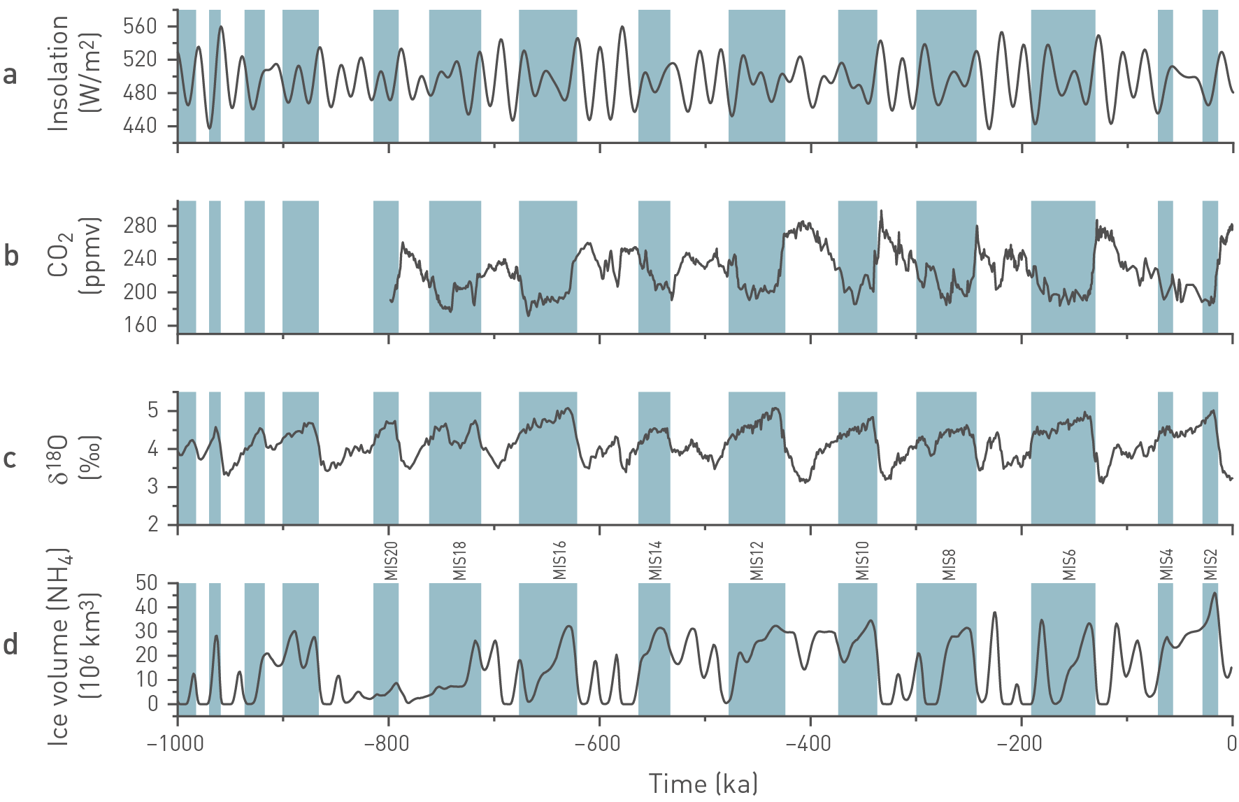
Fig. 6‑11:Comparison of climate proxies for the northern hemisphere during the last million years

(a) Insolation is given for 65°N (July) according to Berger & Loutre (1991). (b) The CO₂ content follows the determinations from Lüthi et al. (2008) and is based on measurements from the EPICA ice core in Antarctica. (c) δ¹⁸O was determined from 57 globally distributed benthic records, collected from the scientific literature (Lisiecki & Raymo 2005). (d) δ¹⁸O was used to calculate a rough estimate of the northern hemisphere ice volume. Blue bars depict even-numbered MIS (periods of glaciations), white sectors correspond to interglacial stages.

The short introduction to climate proxies on a global scale can be viewed as a general guideline to understanding the behaviour of climate and its potential impact at regional and local scales. On a local scale, climate is significantly influenced by e.g. local topographic conditions, distance to the ocean and poles and with respect to prevailing wind directions.

In Northern Switzerland, regional climatic conditions may have influenced the spatial and temporal evolution of foreland glaciations. Up to 15 Quaternary glaciations are assumed to have reached the foreland (Preusser et al. 2011, Ivy-Ochs et al. 2006). Of these, the potentially largest known may have occurred in the past ~ 800'000 years (see also Section 3.5, Section 6.4.1.4 and Fig. 6‑12; Preusser et al. 2011). The advance and retreat of glaciers and their maximum extents for the Birrfeld, Beringen, Habsburg and Möhlin Glacials (Fig. 6‑12) were reviewed by Preusser et al. (2011) and summarised in Nagra (2024k). The Möhlin Glacial is of particular interest because it reached the southern slopes of the Black Forest and is believed to be the most extensive glaciation (MEG) in the Swiss Alpine Foreland during the Quaternary (e.g. Graf 2009b). At that time, the different glaciers (Rhine, Linth, Reuss and Aare – Valais Glaciers) combined and formed a contiguous ice cover. Similarly, during the LGM, glaciers also reached far into the Alpine Foreland, forming a continuous ice cover but with a reduced north-western extent that was smaller compared to that during the MEG. Ice extents of the Habsburg, Beringen and Birrfeld Glacials were smaller than the Möhlin Glacial and, at least during the Habsburg and Birrfeld Glacials, the ice is not believed to have formed a contiguous ice cover (Preusser et al. 2011). The ZNO siting region and partly also NL were covered during LGM-size glaciations, while JO remained ice-free. NL was covered during the Beringen glacial. JO is only covered by exceptionally large fore­land glaciations, such as the Möhlin Glacial (Fig. 6‑12) – these are considered key glacials in future erosion assessments.

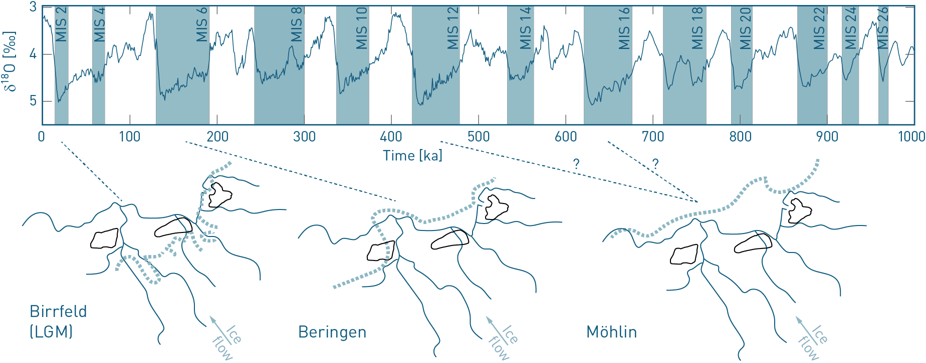
Fig. 6‑12:Key glacials in Northern Switzerland

Glacials (MIS) of the past million years are highlighted together with the key glacials of Northern Switzerland. Sketches show the inferred maximum ice extent (dashed lines) during these times, together with the present-day main rivers and outlines of the siting regions. Ice extent during the LGM covered ZNO and the easternmost parts of NL. The Beringen Glacial is probably associated with MIS 6 and covered ZNO, NL and the easternmost part of JO, and the presumably most extensive glaciation (MEG, Möhlin) covered all three siting regions and is probably associated with MIS 12 or MIS 16 (Preusser et al. 2011).

To understand the regional behaviour of climate and climate-related processes for a specific region of interest, information from local proxies is needed. Such data are often based on analyses of pollen records in (lake) sediments or on measurements such as the δ¹⁸O from dated speleothems (e.g. Luetscher et al. 2021). Proxy information for periods before the LGM is often sparse and more ambiguous but exists, for instance, from the Bergsee (Germany, e.g. Becker et al. 2006, Duprat‐Oualid et al. 2017, Kämpf et al. 2022), Wehntal (Switzerland; e.g. Anselmetti et al. 2010, Dehnert et al. 2012), la Grande Pile (France, e.g. Woillard 1979, Rousseau et al. 2007), and Füramoos (Germany, e.g. Bolland et al. 2022).

Davis et al. (2024) compiled a large number of available pollen data for the LGM, including the Alpine realm, and determined mean seasonal values for temperature and precipitation. Russo et al. (2024) compared these values to climate simulations shown in the following figures. Although the exact timing of events between pollen proxy data and climate simulations is difficult to determine, Russo et al. (2024) showed that climate simulations for the LGM are in good agree­ment with parameter estimations from regional data (see also Nagra 2024j for more detail).

Together with the results of the climate simulations of MIS 4, MIS 6, MIS 8, and MIS 16 and their respective differences, details on the modelling approach can be found in Nagra (2024j). Their comparison suggests that the interplay between mean temperature changes and precipitation changes as well as their seasonality and variabilities are important for the conditions that led to glacier advances into the Alpine Foreland of northeastern Switzerland. Below, illustrations of downscaled simulated climate conditions (temperature, precipitation, and climate classification) are presented for a comparison between pre-industrial (PI) and LGM conditions (Fig. 6‑13). These simulations were further used for the ice-flow modelling (Section 6.3.2). Similar maps for older MIS are documented in Nagra (2024j).

Under pre-industrial conditions (PI) (Fig. 6‑13c, d, g, h), a mean temperature of 8.3 °C (as aver­aged over 10 years in Switzerland) was simulated, which is slightly warmer, in particular during winter, than observations suggest. In this simulation, the difference in temperature between the coldest and the warmest month is 17.5 °C. The yearly mean precipitation is 4.39 mm/day, which is an overestimation compared to observations, again in particular in winter. The difference be­tween the driest and the wettest month, a measure of the variability within a year, is 2.74 mm/day.

The simulated LGM (Fig. 6‑13e, f, i, j) is, on average, much colder than PI, leading to a mean temperature of only -1 °C with a reduced difference of 15.7 °C between the coldest and warmest month. It is also drier than PI, showing a mean precipitation of 3.35 mm/day and a slightly reduced difference in precipitation of 2.65 mm/day over northeastern Switzerland.

Climate classifications can be derived based on such simulations (Fig. 6‑13a and b). While, during the pre-industrial period, most of Switzerland experienced a temperate climate (except for the Alps), during the LGM most of Switzerland saw a polar climate (Fig. 6‑13b).

During the glacials, polar climates (with ice cover or tundra) were likely to have been most pro­minent in Switzerland. Very low temperatures during the glacials would also have caused exten­sive permafrost conditions. Permafrost refers to a condition where subsurface material remains at negative temperatures (frozen) throughout the year and often over very long periods of time (centuries, millennia and more). Permafrost exists today at cold high latitudes and high altitudes. The fact that deep-reaching permafrost during past glacials also existed in wide parts of the European lowlands was documented by the analysis of characteristic deformation features (ice wedge casts and other cryoturbation phenomena) caused by former deep-reaching frost action in unconsolidated sedimentary deposits (Poser 1948, Washburn 1979, Lindgren et al. 2016). During the coldest time intervals, permafrost north of the Alps was continuous, cold (mean annual surface temperature about -5 °C with shorter-term extremes down to -10 °C; Duprat‐Oualid 2019) and reached depths of about 100 to 200 m (Haeberli et al. 1984, Frenzel et al. 1992, Delisle et al. 2003).

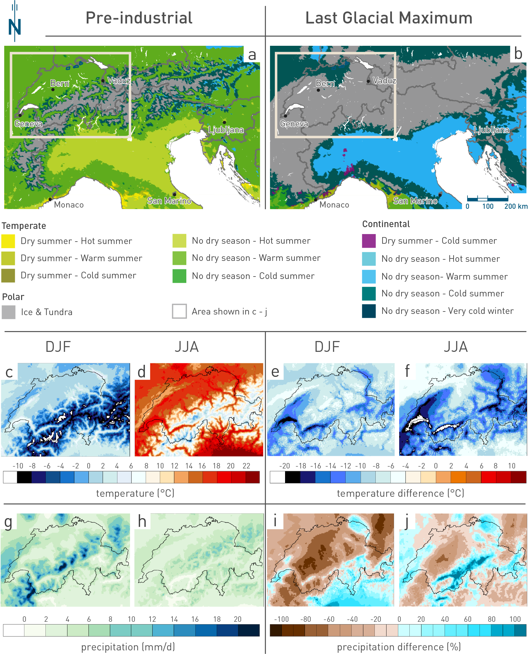
Fig. 6‑13:Temperature, precipitation and climate classification for pre-industrial and LGM climates

The upper panels (a) and (b) show climate conditions from simulations of the pre-industrial period and the LGM (MIS 2), respectively. The climate classifications follow the Köppen classification scheme (Köppen 1918, see Nagra 2024j for more simulations). Note the extent of the polar climate, especially in Northern Switzerland. Below, the figures show simulated mean temperatures for the pre-industrial period in °C for (c) December, January, February (DJF) and (d) June, July, August (JJA), followed by temperature simulation for LGM, visualised as the difference with respect to pre-industrial values in °C (e and f). (g) Simulated precipitation for the pre-industrial period (DJF) as absolute values in mm/day, (h) same as (g) but for period JJA; (i) simulated precipitation for LGM for the period DJF, visualised as the difference with respect to pre-industrial in %; (j) same as (i) but for period JJA.

Simulations of past climates (Section 6.3.1) are used to gain a better understanding of the potential development of glaciers in the Alps, with special focus on the northern central Alps and cor­responding ice flow into the forelands of Northern Switzerland and adjacent Southern Germany. The climate simulations of PI, MIS 2, MIS 4, MIS 6, MIS 8 and MIS 16 and a climate signal proxy are combined to construct a transient climate over past glacial periods. This transient climate is used to force thermo-mechanically coupled, three-dimensional transient ice-flow models to simulate the dynamic evolution and basal conditions of glaciers in the Alps (see Nagra 2024j for further details).

The coupled climate and glacier modelling is used to assess the effects of ice-flow dynamics and related erosion potential in the siting regions during previous glacials. The assessment is based on quantitative criteria that incorporate the physical processes upon which glacial erosion depends (e.g. ice thickness, timing and duration of ice occupation, basal ice temperature, basal sliding velocity and subglacial routing of meltwater). These criteria can be derived from the numerical reconstruction of the ice surface geometry (see Fig. 6‑14), flow dynamics and temperature field of the Alpine Ice Field and, in particular, the Rhine Glacier system (Fig. 6‑16) during past glaciations.

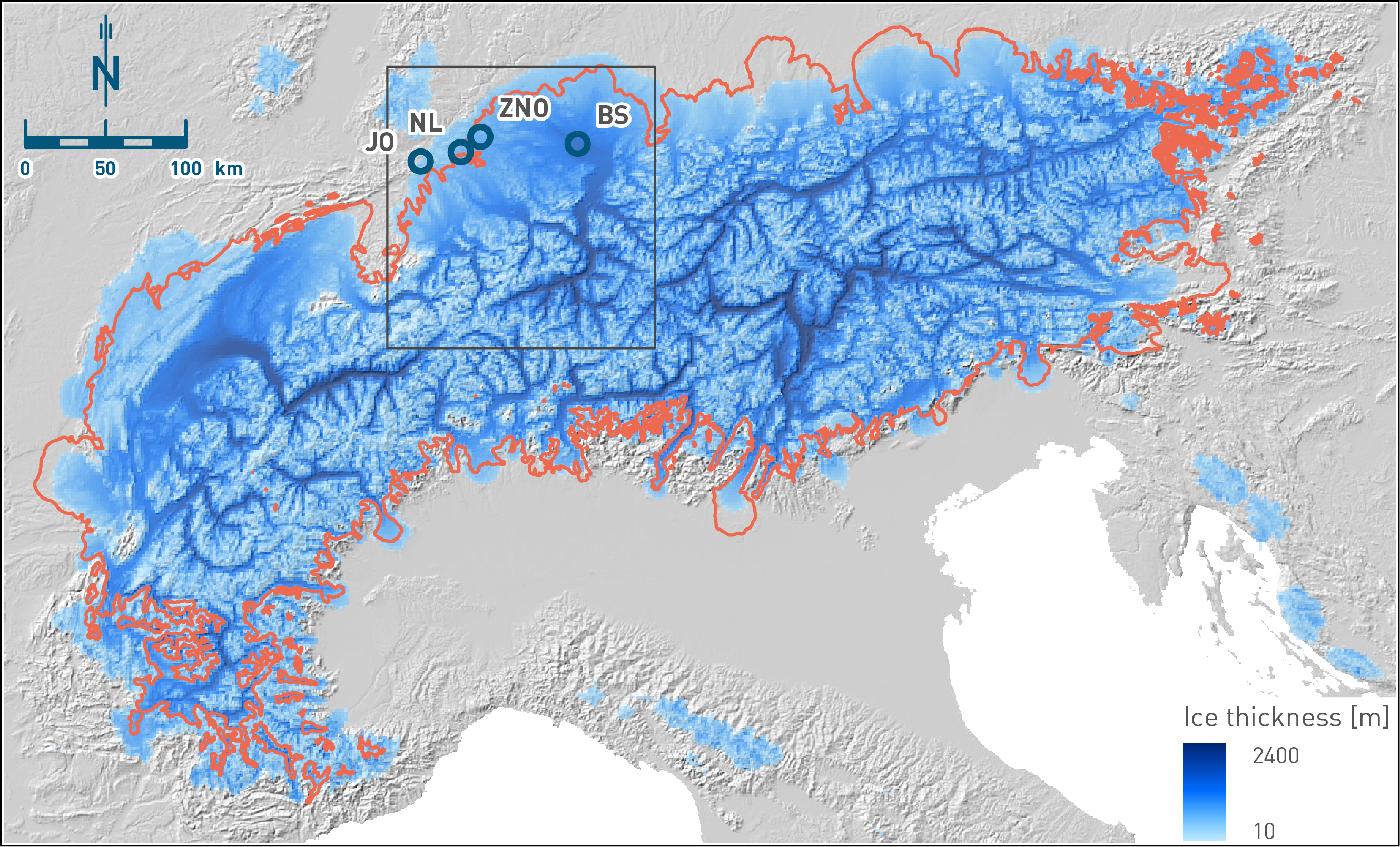
Fig. 6‑14:Modelled maximum ice thickness and extent of the Alpine Ice Field during MIS 2

Geomorphologically reconstructed LGM outline is modified after Ehlers et al. (2011) (red line). Note that different glacier lobes reached their maximum ice thicknesses and extents at different times because fluctuations are controlled by the size of catchments and the resulting inertia of each glacier. The blue circles (JO = Jura Ost, NL = Nördlich Lägern, ZNO = Zürich Nordost, BS = Bodensee) indi­cate locations where ice thickness and duration of ice occupation have been evaluated (Fig. 6‑15). The box shows the Rhine Glacier system (outline of Fig. 6‑16). As basal topography for the model simulations, the publicly available NASA Shuttle Radar Topographic Mission (SRTM, http://srtm.csi.cigar.org/), the Digital Elevation Model (DEM), re‑sampled at 2 km resolution and with major lakes and present-day glaciers removed (Farinotti et al. 2019) are used.

The modelled maximum east to west extent of the Alpine Ice Field during the LGM matches the geomorphological reconstruction of Ehlers et al. (2011) fairly well (Fig. 6‑14Fig. 6‑19). Furthermore, the results show that the flow dynamics of individual modelled glaciers agrees with several indepen­dent key geological observations, including moraine-based maximum reconstructed glacial extents, known ice transfluences and trajectories of erratic boulders of known origin and deposi­tion (Jouvet et al. 2023).

The boxplots in Fig. 6‑15 show the results from different simulations that were carried out as part of a sensitivity study (Nagra 2024j) and suggest a maximum ice thickness of ~ 200 – 400 m and a duration of ice occupation of ~ 1'000 – 3'000 yr in the ZNO and NL siting regions, while JO essentially remained ice-free. Ice thickness and ice occupation duration are significantly larger in the Bodensee region (BS in Fig. 6‑15) due to its more proximal position to the Alpine front.

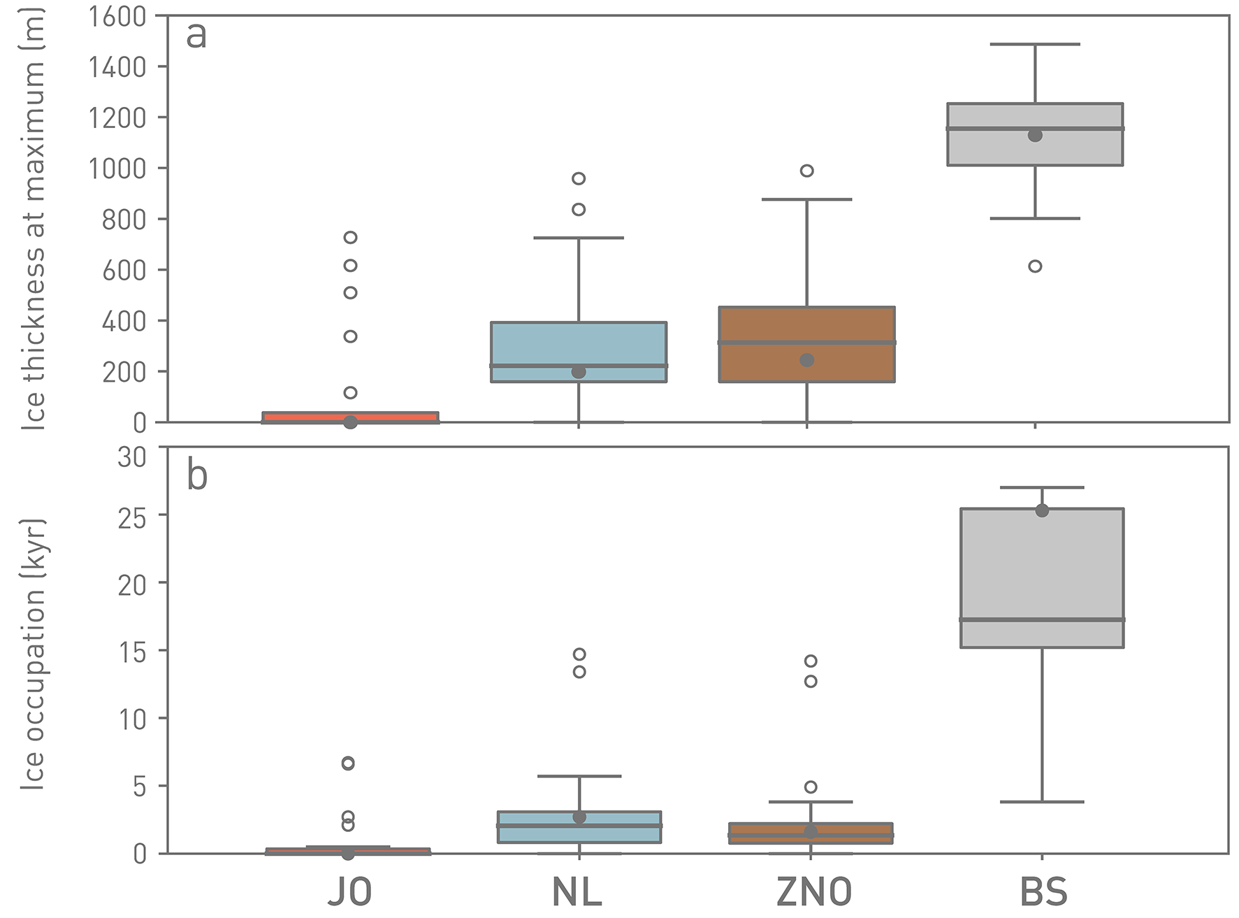
Fig. 6‑15:Boxplots of modelled ice characteristics during the LGM

(a) Maximum ice thickness and (b) Duration of ice occupation. The boxes depict data between the first (25^th percentile) and third quartile (75^th percentile) known as the inter­quartile range (IQR), while the grey line in the box shows the median value (50^th percentile). Black solid points indicate the result from the reference simulation. From above the upper quartile, a distance of 1.5 times the IQR is measured out and a whisker is drawn up to the largest point from the dataset that falls within this distance. Similarly, a distance of 1.5 times the IQR is measured out below the lower quartile and a whisker is drawn up to the lowest point from the dataset that falls within this distance. All other points are plotted as outliers. Data are based on 19 simulations. See Fig. 6‑14 for the locations where ice thickness and duration of ice occupation were evaluated in the Jura Ost (JO), Nördlich Lägern (NL) and Zürich Nordost (ZNO) siting regions as well as for the Bodensee (BS) region.

These results are important for a variety of reasons. Firstly, they provide the boundary conditions for ice dynamics with respect to erosion potential. Secondly, ice loading affects mantle processes (e.g. Wu & Peltier 1982), which in turn cause transient perturbations of the stress field, including effects on uplift pattern and magnitudes (see Section 6.4 and Nagra 2024k) and may influence fault behaviour (see Section 6.2 and Nagra 2024l) and hydrogeological changes (Section 6.5). Assuming an ice density of 917 kg/m³ and mantle density of 3'300 kg/m³, a 400 m ice thickness could produce a lithospheric depression of up to ~ 110 m, if equilibrium is reached. Reaching equilibrium depends, in turn, upon the duration of the ice occupation and the viscoelastic response time influenced by the viscosity of the mantle. These parameters also influence the duration and magnitude of postglacial adjustment. Lithospheric glacial loading and unloading is accompanied by changes in vertical stress (s^v) below the load but deviating horizontal stresses which extend beyond the ice cover (Grollimund et al. 2001, Steffen et al. 2022, Craig et al. 2023).

Basal ice temperature and sliding speed are two key variables that describe basal conditions relevant for glacial erosion (Fig. 6‑16). Glacial erosion occurs where ice is warm-based (not frozen to the ground), which enables basal sliding and thus abrasion. Furthermore, where melt­water is able to flow along the bed, this promotes rapid sliding and stimulates quarrying (plucking) or may directly lead to subglacial meltwater erosion. Simulations for the LGM indicate that basal ice reached the pressure melting point over much of the piedmont lobes of the Rhine Glacier system, and also in the glacial valleys that fed these lobes (Fig. 6‑16a). In the lobes, despite low surface slopes and low basal shear stresses in the Alpine Foreland, sliding dictated the main fluxes of ice, which closely followed bedrock topography. Ice was channelled between bedrock highs along troughs, some of which coincided with glacially eroded overdeepenings (Fig. 6‑16b). These sliding conditions favoured glacial erosion by abrasion and quarrying.

Assuming that the glacial erosion rate scales with the basal sliding speed, the sliding distance calculated by time-integrating the sliding speed (Näslund et al. 2003, Staiger et al. 2005, Yanites & Ehlers 2016) yields a metric for glacial erosion by moving ice. Transient ice-flow modelling of the Rhine Glacier system over the course of the last glacial cycle indicates that the sliding distance is greatest at the base of Alpine valleys where sliding is fastest and where ice occupation time is longest (Fig. 6‑16c). However, the sliding distance does not correlate well with the location of existing overdeepened valleys in the Alpine Foreland (Fig. 6‑16c) owing to the smaller sliding speeds near the ice margin and the short time period during which ice covered the distal foreland (Fischer et al. 2021).

Based on computed time-dependent ice surface elevations, maps of hydraulic potential and associated flow accumulation area are calculated to estimate the location of subglacial water drainage routes and water fluxes (Chu et al. 2016). Time-integration of the flow accumulation area yields a metric for erosion by subglacial water flow. Larger values of time-integrated flow accumulation area indicate zones with significant subglacial water flow that has the potential to enhance sediment removal and increase subglacial fluvial erosion. Results from simulations of the Rhine Glacier system during advance and retreat in the foreland indicate that subglacial water discharge was high and focused along glacial valleys and existing overdeepenings (Fig. 6‑16Fig. 6‑30d), in particular when the water pressure underneath the Rhine and Linth Glacier lobes was close to the ice overburden pressure. These conditions are necessary for subglacial water to remove basal sediments, expose fresh bedrock, and favour further glacial erosion. Knowledge of the location and fluxes of subglacial water drainage is therefore useful for understanding patterns of erosion beneath ice masses that do not otherwise relate to the sliding of ice (Cohen et al. 2023).

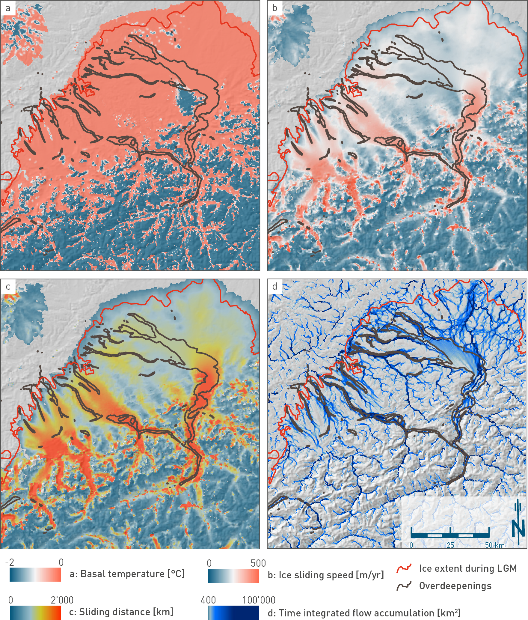
Fig. 6‑16:The Rhine Glacier system and erosion potential at the LGM

(a) Basal ice temperature. (b) Ice sliding speed. (c) Sliding distance calculated by integrating the sliding speed over the course of the last glacial cycle as a proxy for glacial erosion by moving ice. (d) Time-integrated flow accumulation area over 12.8 kyr around the LGM as a proxy for glacial erosion by subglacial water flow (see Nagra 2024j for more details). See Fig. 6‑14 for location. The brown lines denote the outlines of existing overdeepenings. The LGM extent is modified after Ehlers et al. (2011) and is shown by the red lines.

Important characteristics of climate with respect to repository safety are the timing and severity of future glaciations, as the related erosion may reduce the repository overburden thickness and thus modify the properties of the geological barrier (e.g. self-sealing properties, hydraulic con­ductivity; see Sections 6.4.1.4, 6.5). Hence, it is important to simulate future climate and analyse future climate scenarios explicitly with respect to these characteristics.

Parameters for orbital configurations can be calculated accurately for the past and future and are for example reported in Berger (1977, 1978) and Berger & Loutre (1997). However, the future atmospheric CO₂ content cannot be accurately estimated as the additional anthropogenic emis­sions cannot be easily forecast. To accommodate this uncertainty, several emission scenarios were used to cover a range of likely scenarios (Talento & Ganopolski 2021). Palaeo-recon­structions of the past 800 kyr (global mean surface temperature, CO₂ atmospheric concentration and normal­ised global landmass ice volume) were used as part of the training and validation set for the (predictive) model.

The first case is a natural scenario with no additional anthropogenic emissions (0 petagram Carbon [PgC]). This scenario also serves to determine the impact any additional anthropogenic emissions may have. For the period 1750 – 2017, fossil-fuel cumulative emissions and landuse in carbon equivalents are estimated to 660 PgC (Le Quéré et al. 2018). Future projections for addi­tional cumulative emissions might reach between ~ 700 PgC (incorporating fossil-fuel reserves exploitable today) and ~ 3'000 PgC (considering resources that might become exploitable in the future) (McGlade & Ekins 2015). Accordingly, scenarios with additional cumulative emissions of 500, 1'000 and 3'000 PgC are analysed (for more detail see Nagra 2024j).

Talento & Ganopolski (2021) defined the occurrence of full glacial conditions and large glaciations at the 0.5 and 0.8 value of the normalised global landmass ice volume, respectively (see Fig. 6‑17 for best solution scenarios). With respect to the long-term geological evolution of the repository sites, the main interest is in the potential future timing of large glaciations, as they may reach the Alpine Foreland. This timing is expected to correspond to the peaks above the 0.8-unit ice volume threshold in Fig. 6‑17 (note that ~ 1 corresponds to the global equivalent of LGM ice volume).

In general, the higher the carbon concentration in the atmosphere, the later the next glaciation will occur (Fig. 6‑17 for best solutions). In the natural scenario (E = 0 PgC), the next full glacial condition is simulated to peak around ~ 110 kyr (Fig. 6‑17a). For the low emission scenario (E = 500 PgC), the next full glacial condition is postponed by ~ 90 – 100 kyr compared to the natural scenario, with a peak at ~ 220 kyr and simulated ice volumes of 0.8 (Fig. 6‑17b). For the intermediate emission scenario (E = 1'000 PgC), full glacial conditions only occur the first time at ~ 650 kyr (Fig. 6‑17c). Finally, with a cumulative emission of 3'000 PgC, simulations indicate mostly ice-free conditions for the next 800 kyr (Fig. 6‑17d). In this scenario, full glacial condi­tions are not expected to occur before 850 kyr. Once the first larger glaciation has occurred, all scenarios show a cyclicity of approximately 100 kyr, similar to the glacial/interglacial cycles, established after the Mid-Pleistocene Transition; see Section 3.5).

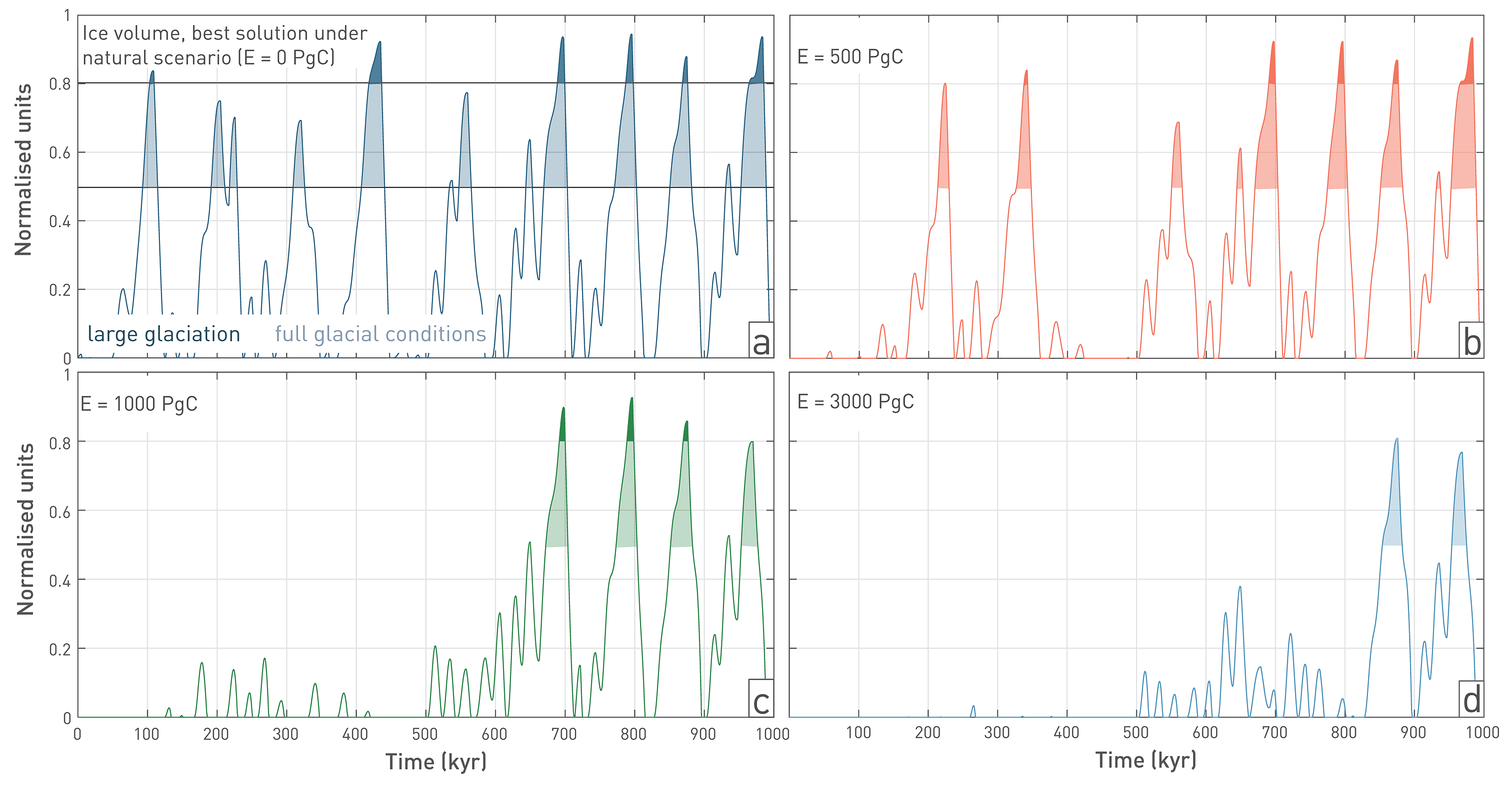
Fig. 6‑17:Future climate simulations based on orbital configurations and different Anthro­po­genic CO₂ scenarios

The plots show the "best solution" simulations of global ice volume as proxy and are redrawn from Talento & Ganopolski (2021), using normalised global landmass ice volume as proxy for future glaciations. A value of 1 refers to approximately the same amount of ice as deter­mined for the peak of the LGM. Full glacial conditions are suggested to occur at 0.5 units (filled parts), while a value of 0.8 may suggest a large glaciation (darker filled peaks). With respect to the long-term geological evolution of the repository sites, such large glaciations might reach the North Alpine Foreland. (a) Scenario with zero anthropogenic CO₂ emis- sions. A large (potentially reaching the North Alpine Foreland) glaciation occurs only after ~ 100 kyr from now. (b) Scenario with cumulative emissions of 500 PgC. In such a scenario, the next glacial inception is significantly delayed, with the next large glaciation occurring only after ~ 200 kyr. (c) The 1'000 PgC scenario considers consumption of all presently exploitable fossil fuel reserves and will further delay future large glaciations. (d) 3'000 PgC represents a worst-case scenario, including fossil fuel reserves that might become exploitable in the future.

Another important characteristic is the prevailing climate during the glacials and interglacials because it determines living conditions for humans directly above, or in the vicinity of, the repo­sitory.

Following the Köppen climate classification scheme (Köppen 1918), a typical climate at the start of a glaciation is a polar climate, followed by continental and temperate climates. Polar, conti­nental and temperate climates have all occurred in the past and are well documented using proxy data and simulations (Nagra 2024j), and it is reasonable to assume that they are also representative for future glacial/interglacial cycles. At the height of an interglacial period, Switzerland may also experience a warmer-drier climate, especially if high carbon emissions are assumed. Simulations of the IPCC using Scenario RCP8.5, which is approximately equivalent to the 3'000 PgC scenario, predict warm-temperate climates for Switzerland by 2100. These climates are defined as having a mean temperature during the coldest month above 0 °C and above 22 °C for the warmest months, while 8 months have mean temperatures above 10 °C (IPCC 2023). A dry climate is defined as having very little precipitation and very high average monthly temperatures throughout the year. Currently, most of Spain experiences temperate to dry climates. According to Beck et al. (2018), the dry climate will advance north-eastwards in the next 100 yr and reach the Pyrenees while arid conditions are expected in parts of Spain. Under normal low or natural emission scenarios, a dry climate is not to be expected in Switzerland during a glacial/interglacial cycle. However, with continued carbon emissions and subsequent climate change a warmer-drier climate cannot be ruled out that, at least in the high-emission scenarios, such a dry climate may occur even in Switzerland in the future.

Climate is an important driver for erosion and has direct hydrogeological and geomorphological effects, in particular related to glacial erosive and depositional processes. Considering the present-day climate assessment and projected conditions regarding future climate states in the Alpine realm, the conclusions are:

• Glacials are of fundamental importance with respect to erosion processes in Northern Switzer­land.

• The palaeoclimatic record and simulations of past Quaternary climates show that the global as well as the local climate evolution of Northern Switzerland was dominated by a succession of glacial/interglacial cycles. Before the Mid-Pleistocene Transition (between 1.25 and 0.7 Myr), these cycles lasted approximately 41 kyr, while after the transition 100-kyr cycles became dominant.

• Using the geological and geomorphological record, especially for the last glacial/interglacial cycle, the ice extent in the greater Switzerland area can be mapped and simulated. Glaciers reached far into the Alpine Foreland, repeatedly covering Northern Switzerland.

• The ZNO siting region and partly also NL were covered during LGM-size glaciations, while JO remained ice-free. ZNO and NL were covered by the Beringen Glacial. JO is only covered by exceptionally large foreland glaciations, such as the Möhlin Glacial.

• During the coldest time intervals, permafrost north of the Alps was continuous, cold (mean annual surface temperature about -5 °C with shorter-term extremes down to -10 °C) and reached depths of about 100 to 200 m

• Ice-flow modelling allows estimation of the erosion potential in Northern Switzerland during foreland glaciations; basal ice temperature and sliding speed are key variables for glacial erosion. Ice was channelled along troughs; these sliding conditions may have favoured glacial erosion. High subglacial water discharge is key to removing basal sediments, exposing bedrock and favouring further glacial erosion.

• A maximum ice thickness of ~ 200 – 400 m and a duration of ice occupation of ~ 1'000 – 3'000 yr in ZNO and NL were simulated and are expected for future foreland glaciations.

• Insolation is one of the main climate drivers and can be calculated accurately for the future. The atmospheric CO₂ concentration has a very strong influence on the timing and severity of future glaciations. Only if the greenhouse gas concentration is reduced to pre-industrial levels, will the next glaciation be expected to occur at around 100 kyr after present. An additional 500 PgC will postpone the next larger glaciation to > 200 kyr. Even higher total carbon emissions will move the onset of the next glaciation further into the future.

• After a glaciation, the climate warms, and climate conditions change from a polar climate (Switzerland largely covered by ice and/or permafrost conditions) towards a continental, temperate or potentially an even warmer-drier climate.

Erosion is the main process that can reduce the protective overburden thickness needed for sustained barrier functions (Section 6.1.2). In addition to information on the drivers of erosion (Sections 6.2 and 6.3), this section builds on Sections 3.4.5 and 3.5 and provides the key facts of past landscape evolution that allow a first-order assessment of past erosion processes and rates. To project these rates and processes under consideration of uncertainties into the future on a one-million-year timescale, a hybrid-probabilistic framework was established.

Section 6.4.1 summarises the main evidence needed to understand the Quaternary landscape evolution. It builds on site investigations (Section 2.4), but also incorporates general process understanding.

This information was used to derive probability distributions and arguments for parameters to be used in subsequent erosion modelling and assessments (Section 6.4.2). The main results and asso­ciated line of reasoning for each separate erosion process are presented briefly in Section 6.4.3.

Section 6.4.4 shows the combined results of the erosion assessment for the future one-million-year time frame. Discussed are the remaining overburden thickness for the expected geological evolution as well as, to show the robustness of the repository, the probability of repository excava­tion.

A summary of the main results is given in the conclusions of Section 6.4.5.

Tectonism and climate changes during the Quaternary have shaped the present-day landscape of Northern Switzerland (Chapter 3, Sections 6.2 and 6.3). The main erosion processes that are involved are the combined action of rivers and especially the drainage evolution of the Aare – Rhine River system, as well as erosion and sedimentation by repeated large foreland glaciations. These processes, in turn, control topographic slopes and mass movements, thus driving denu­dation of the topography.

The respective landscape forms derived from fluvial incision, evolution of hillslopes, and deep glacial erosion provide important geomorphic reference markers (Schnellmann et al. 2014). These markers allow the landscape to be divided vertically into different geomorphic compartments. Based on these markers, the geomorphic constraints at the respective repository sites can be determined and an assessment of future erosion made (Section 6.4.3). In the following, the three compartments and the main differences affecting the siting regions are briefly described (for more details see Nagra 2024k).

The main reference horizon, i.e. first landscape compartment, constitutes the local erosion base – the locally deepest fluvial incision level in bedrock (Fig. 6‑18b). The local ersosion base is a virtual surface that is spanned between the thalwegs of the main river channels of the Rhine, Aare, Limmat, and Reuss and declines towards WNW. Some of these thalwegs are filled with sediments so that the bedrock interface defines the thalweg depth, and the local ersosion base is lower than the present-day river bed (see Pietsch & Jordan 2014 for more details¹⁴). No local river can signi­ficantly incise below this level. The local erosion base affecting the siting regions is gently inclined towards the WNW and is mainly defined by the paleochannels of the Rhine, Aare, Limmat and Reuss Rivers (Fig. 6‑18b). The Quaternary fluvial incision history of Section 6.4.1.2 describes the past evolution of the local erosion base.

The local erosion base (LEB) separates the rocks (bedrock and unconsolidated sediments) above (here called local topography, Fig. 6‑18c) from the unconsolidated Quaternary sediments that fill the glacially overdeepened basins (glacial overdeepenings, Fig. 6‑18d) below.

Section 6.4.1.3 describes processes and rates that reflect the evolution of local topography in selected areas of Northern Switzerland and Section 6.4.1.4 summarises the Quaternary glacial history that led to deep glacial erosion and overdeepened basins. More details can be found in Nagra (2024k).

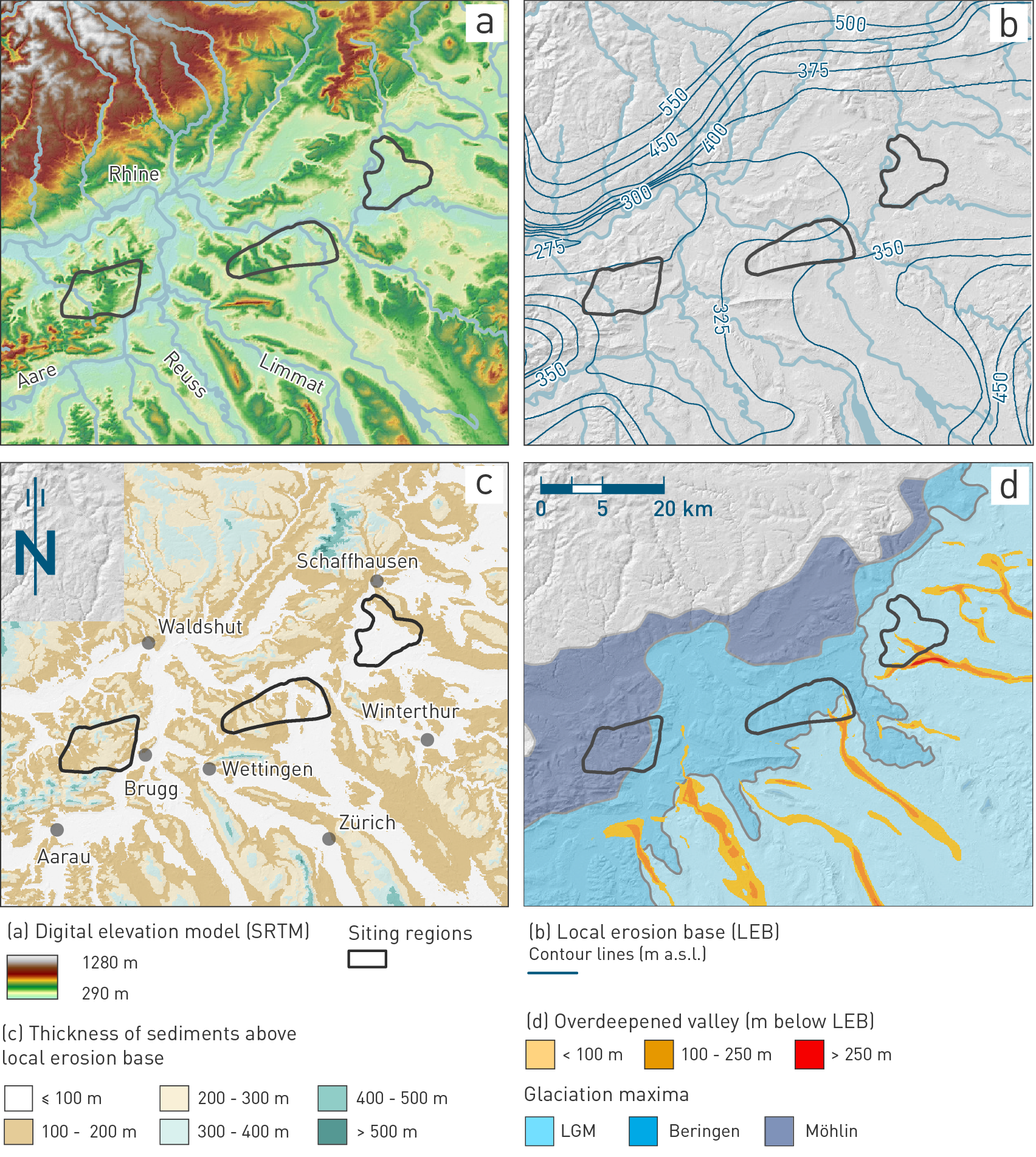
Fig. 6‑18:Maps showing the main landscape compartments around the siting regions

(a) Digital elevation (NASA Shuttle Radar Topographic Mission SRTM, Digital Elevation Model) on a hillshade model showing the relief distribution around the siting regions and main rivers. (b) Contours of local erosion base (LEB) as derived by Pietsch & Jordan (2014). (c) Colour-coded thickness of local topography, i.e. the sedimentary rocks and unconsoli­dated Quaternary sediments above the LEB. (d) Ice extents of the three Quaternary key glacials (blue colours, see Section 6.4.1.4) and distribution and depth of glacial over­deepenings (orange colours). The siting regions are plotted in each subfigure for comparison.

The main parameters driving fluvial incision are uplift/subsidence, climate-driven water and sediment flux, and erodibility, with natural feedback between them.

Climate-driven water and sediment flux

The glacial/interglacial cyclicity (Section 6.3) has a major impact on the spatiotemporal sediment production and transport in Alpine source areas and their forelands (e.g. Antoniazza & Lane 2021). Sediment yield may be highly variable during phases of glacier advance, retreat, and readvance for instance. Antoniazza & Lane (2021) describe the highest sediment availability during early phases of glacial retreat and re-advance, before the sediment sources become exhausted at later stages.

Hinderer (2003) provided a source-to-sink case study from the Alpenrhein and Bodensee area, covering the Late Pleistocene and Holocene. They propose temporal storage of sediment in the source areas and the foreland during glacials. The highest sediment flux instead was observed during early melting (10× higher flux during the Late Pleistocene when compared to today). Importantly, the Bodensee as a large periglacial lake constitutes an efficient sediment trap and decouples further sediment flux into the foreland and the Hochrhein area (Hinderer 2003).

Upon filling of the Bodensee, incision in the Hochrhein is limited, because bedload is trapped within the lake and is not available as tools for fluvial impact erosion. The largely preserved knickpoint of the Rhine Falls seems indicative for this process. When bedload tools become available, it is expected that the local incision will strive towards equilibrating the longitudinal profile of the Hochrhein. However, at this point, further sediment flux from the Alpenrhein and the source region is no longer inhibited and large sediment supply may result in the opposite cover effect, i.e. shielding the riverbed from further vertical downcutting.

Rock uplift and stream piracy – process and Quaternary history

Rock uplift and subsidence of any landscape is mainly driven by neotectonic activity and/or iso­static compensation to mass redistribution by glacial processes (erosion and deposition). The effects of these processes dictate rates and locations of incision and sediment accumulation and thus can cause changes in river profiles (steepening, knickpoints), catchment changes by piracy, and variability in strength of the exposed rocks.

The influence of tectonic domains on the river profiles of the Aare and Rhine were explained in Section 6.2.2. Most important is the rock uplift of the Alpine Foreland. However, Rhine – Danube catchment competitions can also cause a sudden significant drop of the baselevel. As highlighted in Section 3.4.5, the past evolution of the Aare – Rhine River system occurred in several phases of drainage reorganisation that resulted in significant baselevel drops between tens of metres and up to several hundred metres (see Fig. 3‑11 in Section 3.4.5). The present-day longitudinal profile of the Rhine is significantly shorter than that of the neighbouring Danube, which causes the Rhine catchment to grow at the expense of the Danube to achieve geometric equilibrium of the water­sheds (e.g. Winterberg & Willett 2019). This relationship is illustrated in Fig. 6‑19. The drainage divide has successively shifted further east as this process progresses. Importantly, fluvial geometric imbalance is often associated with variable erosion (incision) rates, and those rivers and tributaries that gain watershed experience an increase in rates (e.g. Willett et al. 2014). Most likely, the main pulse of increased incision based on past reorganisation has already propagated through the Hochrhein (range of the siting regions). This hypothesis is supported by the observation that the Hochrhein has attained an overall along-river gradient that is comparable to the Rhine River section draining the Upper Rhine Graben. Former river gradients need to be interpreted with care due to the possibility of tectonic tilting, but were still steeper than today, possibly showing a gradual adjustment since the emplacement of the Höhere Deckenschotter (HDS; Fig. 6‑19b). The relatively low gradients today suggest also that similar drainage changes in the future will most likely lead to minor if any increased incision. Any large events of fluvial incision in response to drainage reorganisations are therefore not to be expected within the next one million years.

The Quaternary incision history, which is an important parameter for evaluating future incision, probably reflects a combination of rock uplift and piracy-related baselevel lowering. In the following paragraph, the Quaternary incision history is briefly summarised based on four main morphostratigraphic units with fluvioglacial sediments (Fig. 6‑20) that have been differentiated in the Swiss Alpine Foreland: Höhere Deckenschotter (HDS), Tiefere Deckenschotter (TDS), Hochterrasse (HT), and Niederterrasse (NT) (Graf 1993; Preusser et al. 2011), see also Section 3.5 and Nagra (2024k).

The HDS and TDS units are characterised by complex internal geometries (cut-and-fill sequences, see inset in Fig. 6‑20), in which several depositional phases can be distinguished, for example based on clast petrography and orientation (Graf 1993). These deposits reflect protracted deposi­tional phases, largely in proximity to former glaciers. In addition, interglacial overbank deposits occur for example in the HDS (Hasli Formation) at Irchel (Thew et al. 2024, Bolliger et al. 1996) and in the TDS at Hungerbol (Graf 2009a). The base of the HDS and TDS units may locally differ by several decametres (usually between 30 and 100 m), thus reflecting a period of net bedrock incision between the depositional phases (see also Fig. 6‑19b). While the base of the relict HDS deposits is predominantly more or less planar, the TDS deposits are associated with pronounced channel forms. Accordingly, their base is highly irregular and has considerable relief differences (see for instance Fig. 6‑20, inset). The incision between HDS and TDS accumulation might have been caused by increased subsidence of the Upper Rhine Graben, increased uplift of the external Alpine Foreland (Preusser et al. 2011), and/or by re-routing of the Alpenrhein from the Danube towards the ‘recent’ Rhine system through the Rhine Graben (see Section 3.4.5, Fig. 3‑11); Claude et al. 2019). Age control of these units has improved considerably, but is still debated depending on different geochronometers (see Fig. 6‑20a and Nagra 2024k for more detail).

Two main phases of sediment accumulation following bedrock incision occurred after the deposition of the HDS and TDS units (Fig. 6‑19b and Fig. 6‑20). The morphostratigraphically next lower level (Hochterrasse, HT) is located about 50 to 200 m below the TDS level, depending on the region. The difference significantly increases from west to east and from north to south (Preusser et al. 2011). It has been argued that this significant drop of the local erosion base after TDS accumulation could potentially be associated with the Mid-Pleistocene Transition (MPT, see Section 3.5). Preusser et al. (2011) speculated that these changes, including glaciations extending into the Alpine Foreland, might have led to reorganisation of the major drainage system. Accordingly, the Alpenrhein at the location of the Bodensee changed its course from previously draining towards the Danube towards a new Hochrhein direction.

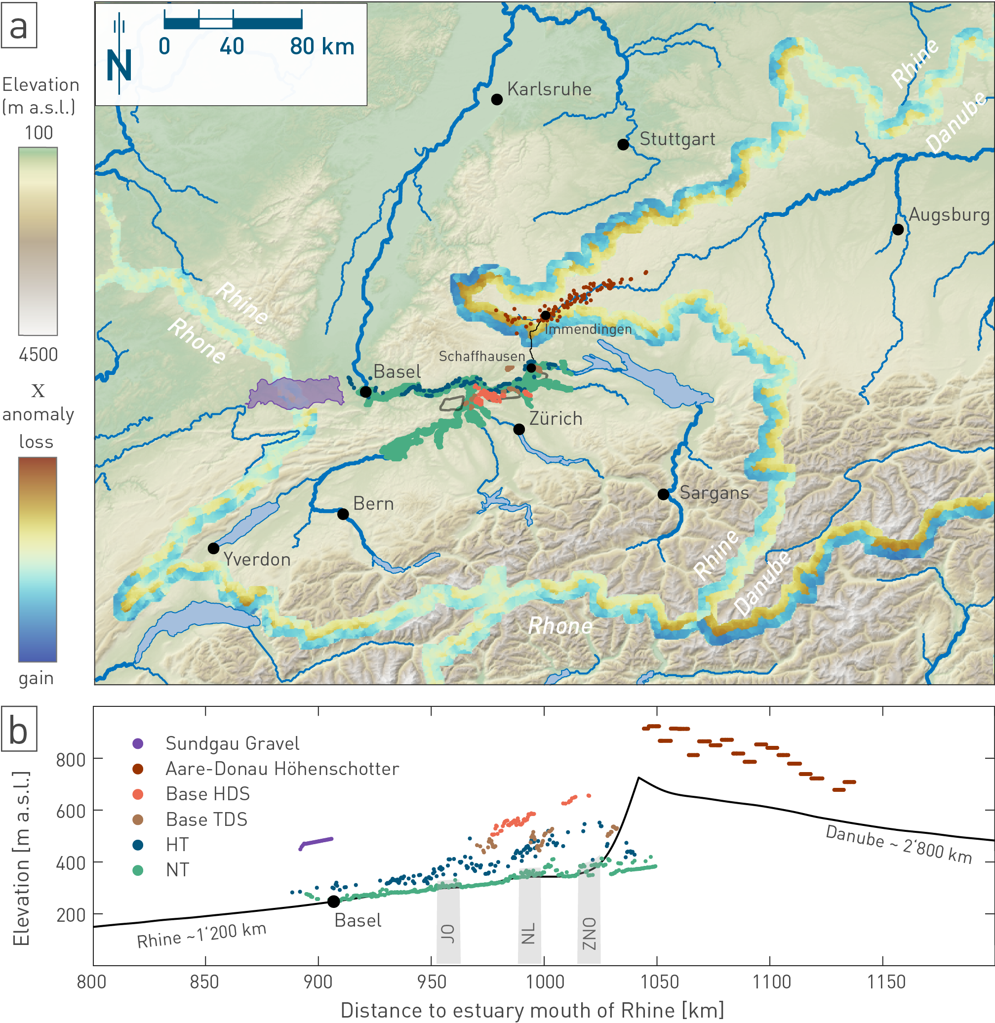
Fig. 6‑19:Catchment competition between the Rhine and Danube watersheds and drainage reorganisation

Digital terrain model (a) with main river courses and their catchments. The drainage divide of the Rhine catchment is outlined by a visualisation of the direction of future catchment growth (calculation of a parameter , e.g. Willett et al. 2014). The  anomaly quantifies the differences in the parameter  on either side of the divide. The  parameter is calculated for the river network and then projected onto the main upslope divides. Blue values indicate low  values and thus potential future gains in drainage area, whereas red values indicate potential losses. Sharp cross-divide contrasts thus highlight regions of potential future drainage reorganisation. In turn, similar anomaly values on both sides suggest stable divides. Also shown are locations of major fluvial to fluvioglacial deposits, see legend in (b) for colour-code. These deposits constitute important marker horizons for the past evolution of the drainage system. (b) Simplified comparison of partial longitudinal river profiles of the Rhine and Danube artificially connected along the black line between Immendingen and Schaffhausen in (a). The distance along the Rhine to the North Sea is remarkably shorter than the distance of the Danube to the Black Sea, resulting in a higher altitude of the Danube system. This difference resulted in a significant erosional pulse after capturing the Alpine-to-Danube River reaches and diverting them into the Rhine. The approximate position of the siting regions is indicated by the grey-coloured bars. The level of the Rhine is already clearly lowered at these positions (also visible from vertical the position of the fluvioglacial deposits) and is part of an equilibrated longitudinal profile, which suggests that the main pulse of the incision caused by the capture has already migrated through the Hochrhein and passed the repository sites.

On a more local scale, repeated drainage shifts were also observed during HT sediment accumu­lation. In an early phase, the higher Thur Valley drained via Stammheim, Schaffhausen and Klett­gau towards Basel (northern HT occurrences), while the river’s course via Eglisau and Koblenz (southern HT occurrences) probably became established only after the penultimate (Beringen) glaciation (Fig. 6‑20; Graf 2009a). Clast provenance additionally provides evidence for an early drainage between Walensee and Klettgau (Graf 2009a). The vertical difference between the elevation of the deepest fluvial channel and the highest mapped gravel surface within the morpho­stratigraphic Hochterrasse unit can attain more than 100 m.

The lowest bedrock elevation attained prior to Hochterrasse deposition (e.g. Graf & Burkhalter 2016) is still considered the lowest regional level and constitutes the basis for the main reference used in evaluating future incision, the so-called local erosion base (see Section 6.4.1.1). Based on luminescence ages of the fluvial channel deposits, this depositional phase may fall within MIS 6 (onset ca. 190 ka ago, minimum age; e.g. Lowick et al. 2015).

No deeper vertical bedrock incision took place after MIS 6. The even younger Niederterrasse deposits were deposited onto the (partly incised) previous fill of Quaternary sediments or on bedrock at higher or approximately equal positions to the HT. In many places, these deposits are currently being incised by the Aare and Rhine Rivers and their tributaries (Fig. 6‑20), locally more than 30 m (Nagra 2024k). About 14 m of postglacial incision (post-Würm glaciation) into Nieder­terrasse sediments are observed in the southern Upper Rhine Graben (Hillebrand & Frings 2017).

Mean values of incision rates derived for bedrock incision after HDS or TDS deposition (base HDS or base TDS to local erosion base, respectively), ranged between ~ 0.1 and ~ 0.3 mm/yr (see Section 6.2.2 and Nagra 2024k). This is based on simplified assumptions: firstly, the elevation of base of the deposits (i.e. the bedrock elevation) is used, to address the net lowering of the local baselevel over time, independent of intermediate aggradation phases. Secondly, it is assumed that the age range reflects the deposition at a late stage, i.e. shortly before the subsequent incision. Combining an age derived from sediment deposits accumulated up to several tens of metres with the elevation of the bedrock marker below these sediments requires the third assumption: a "quasi-instantaneous" incision through the unconsolidated Quaternary deposits.

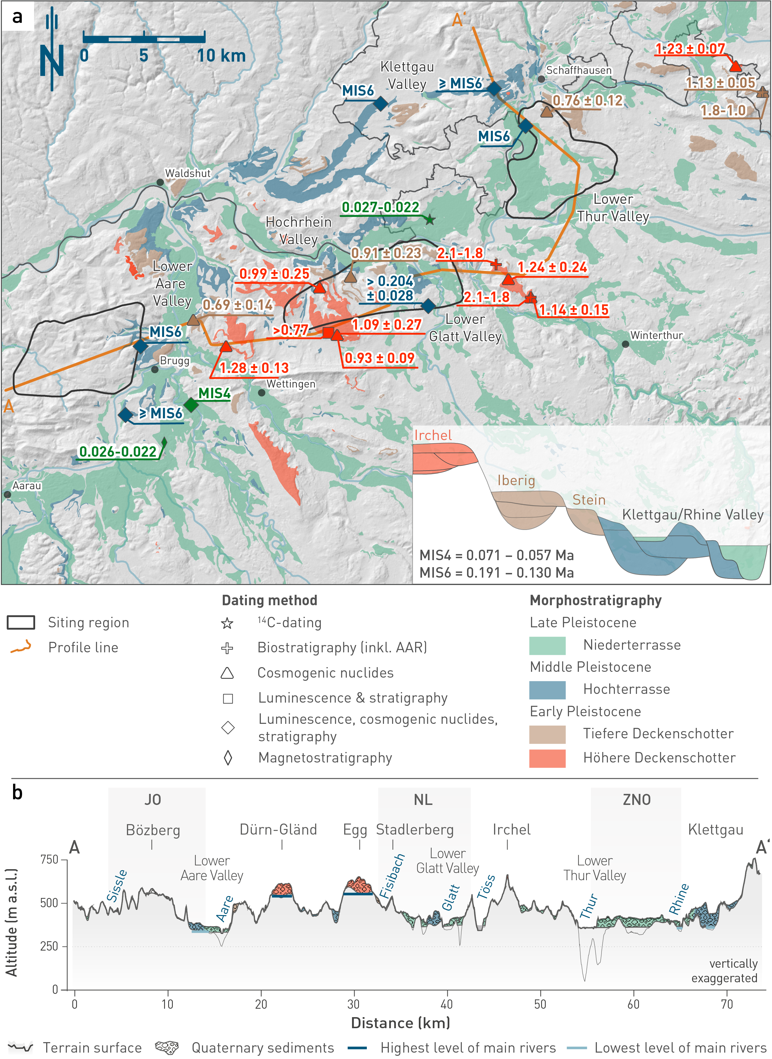
Fig. 6‑20:Morphostratigraphic units in Northern Switzerland with selected age information

(a) Ages are colour-coded according to the morphostratigraphic unit of the respective deposits and listed with symbols according to dating method: biostratigraphy (Thew et al. 2024), AAR (Penkman et al. 2024), magnetostratigraphy (Scheidt et al. 2023), luminescence & stratigraphy (Mueller et al. 2024, Gegg et al. 2023, Kamleitner et al. 2023, Gegg 2021, Mueller et al. 2020, Gaar et al. 2019, Buechi et al. 2017, Lowick et al. 2015, Reber et al. 2014, Dehnert et al. 2012), cosmogenic nuclides (Dieleman et al. 2022a, Grischott et al. 2020, Knudsen et al. 2020). Inset shows sketch of morphostratigraphic relationship with complex cut-and-fill sequences within each unit (based on Graf 2009a). (b) Simplified profile (see a for location) through the siting regions and crossing several Deckenschotter deposits. Note highest fluvial level (dark blue) and lowest level (light blue).

Lithological control

Generally, two main counteracting processes are important for bedrock incision: (1) the "tool effect" when bedload (the tools) is available to erode the bed by impact, abrasion, or quarrying, and (2) the "cover effect", when the riverbed is protected from erosion by a critical sediment cover (e.g. Turowski et al. 2007). Erodibility, which defines the rock resistance against erosion¹⁵, has an impact on sediment production and discharge, grain size, and bedload in the channel. The main influences on erodibility, in turn, are lithological contrasts, often defined by their rock com­pressive and tensile strengths (e.g. Fig. 6‑21a, c).

The lithologies that form the stratigraphic column in Northern Switzerland comprise variable degrees of rock resistance (erodibility) with respect to the influence of fluvial impact erosion, as determined by abrasion mill experiments (Fig. 6‑21b; Turowski et al. 2023). Resulting erosion rates derived from these experiments varied over about six orders of magnitude. Uncertainties scale with measured erosion rates.

Erosion rates measured on samples from the same lithostratigraphic unit revealed variability, most notably (for the given dataset) within the Lower Freshwater Molasse Group. Nevertheless, as expected, weakly consolidated sandstones or mudstones show the highest erosion rates and lowest tensile or compressive strength, and crystalline rocks such as granite tend to show the lowest erosion rates and highest tensile or compressive strength (Fig. 6‑21).

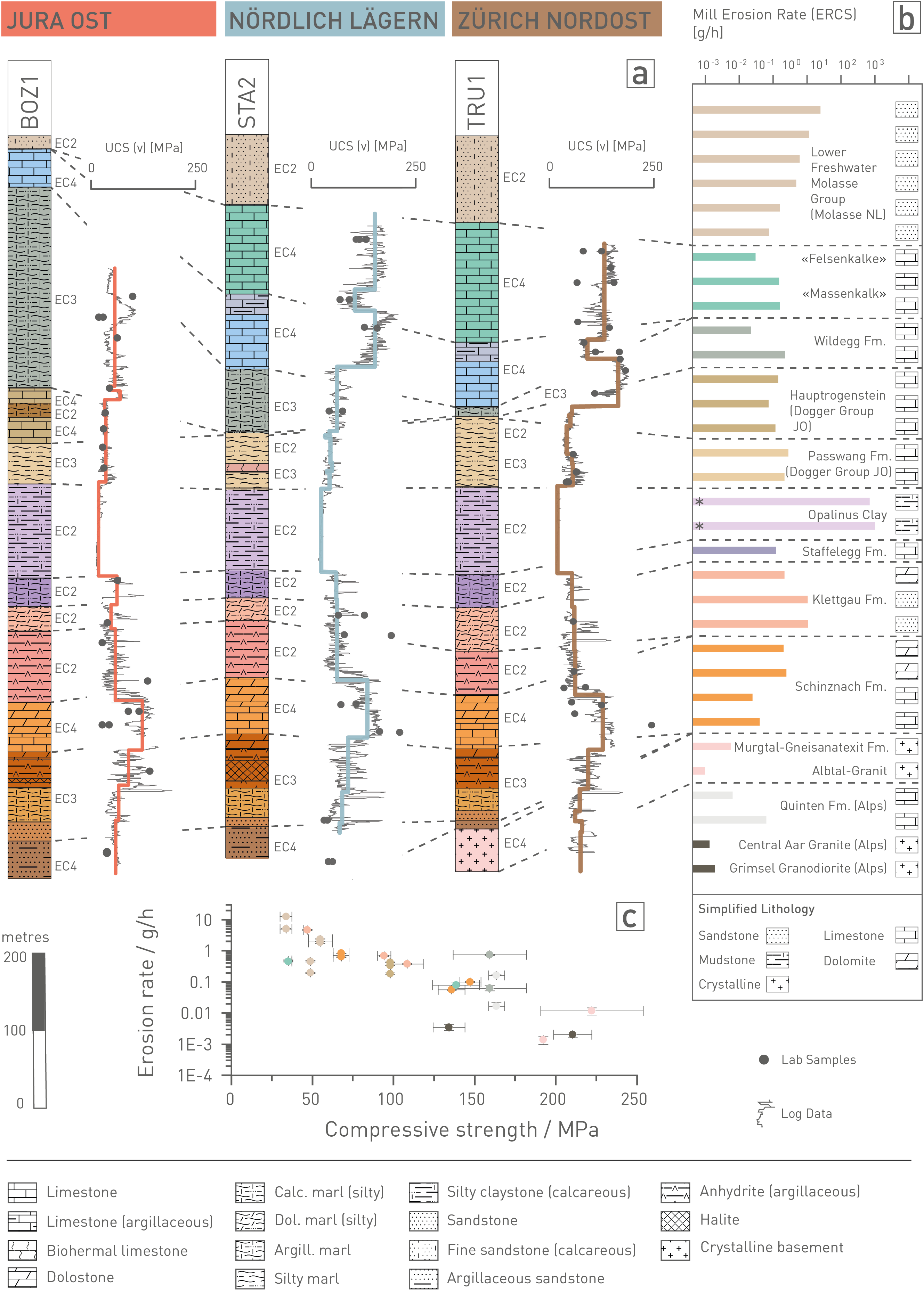
Fig. 6‑21:Unconfined compressive strength and abrasion mill erosion rates as quantitative indicators of bedrock erodibility

(a) Stratigraphic columns based on the BOZ1, STA2, and TRU1 boreholes with measured and estimated unconfined compressive strength (UCS) from selected deep boreholes in the three siting regions. Measured data points are based on core samples tested in the laboratory (Dossier IX in Nagra (ed.) 2022a, 2022c, 2021c). Continuous curves were approximated by combining the laboratory measurements with borehole log data from Nagra (2024m). Erodibility classes (EC) along the stratigraphic columns reflect the abstraction of the litho­stratigraphic units as used for erodibility-related parameterisation in Model B of the erosion assessment model cascade described in Section 6.4.2.3 (Fig. 6‑29). Quaternary deposits (not displayed here) are assigned to EC 1. (b) Relative erodibility in fluvial impact erosion as represented by erosion rates from abrasion mill experiments (Turowski et al. 2023; see further details there). Measurements were conducted on intact rock samples in the laboratory (ERCS method = erosion rate from the concentration of solids), from lithostratigraphic units as labelled. Asterisks denote results for highly erodible Opalinus Clay samples, where devia­tions from the standard experimental procedure were necessary. Samples were collected from surface outcrops, except for the Opalinus Clay and Alpine crystalline rock samples that were taken from the FMT and GTS rock laboratories, respectively. Due to technical limitations, there is a sampling bias towards harder rock types. This is mostly important for more heterogeneous formations, where samples focus on the harder beds (e.g. cemented sandstone layers in the Molasse units and limestone layers within the Wildegg Formation). Note the simplified lithological classification. (c) Strong negative correlation between abrasion mill erosion rate and UCS is suggested by paired laboratory measurements by Turowski et al. (2023). Error bars are only discernible if larger than the data point symbols. Colours cor­respond to figure part (b). Note that data for the Opalinus Clay and the Passwang Formation from (b) are missing in (c) because of a lack of UCS measurements on these samples.

An impressive example of the effect of variable erodibility on a river’s longitudinal profile is the Rhine Falls knickpoint that is located within resistant limestones. However, besides the litho­logical contrast, the present-day incision efficiency needed to erode this knickpoint seems to be hampered by trapping of the Alpine sediments (i.e. the tools for efficient bedrock erosion) within large glacially overdeepened lakes, e.g. the Bodensee. Accordingly, a major control on the tool and cover effects and thus on the sediments and fluvial dynamics of Northern Switzerland is the glacial/interglacial cyclicity.

Channel-hillslope coupling

Fluvial incision and deep glacial erosion processes determine the pace at which hillslopes respond to baselevel changes. Topographic slope stability depends for instance on the slope angle, con­trolled by the fluvial baselevel and associated mass movements. Thus, the nature of channel-hill­slope coupling will drive denudation of the topography (Fig. 6‑22a). This coupling also provides the link between the landscape compartments that define the local erosion base and local topography (see Section 6.4.1.1).

Rock properties (e.g. rock strength, fracture spacing, orientation of discontinuities with respect to slope), vegetation cover, and climate factors add to the control on hillslope stability or failure and can influence denudation rates. The distinct morphology and different geomorphic process rates that define a landscape need to be incorporated into any future assessment of erosion.

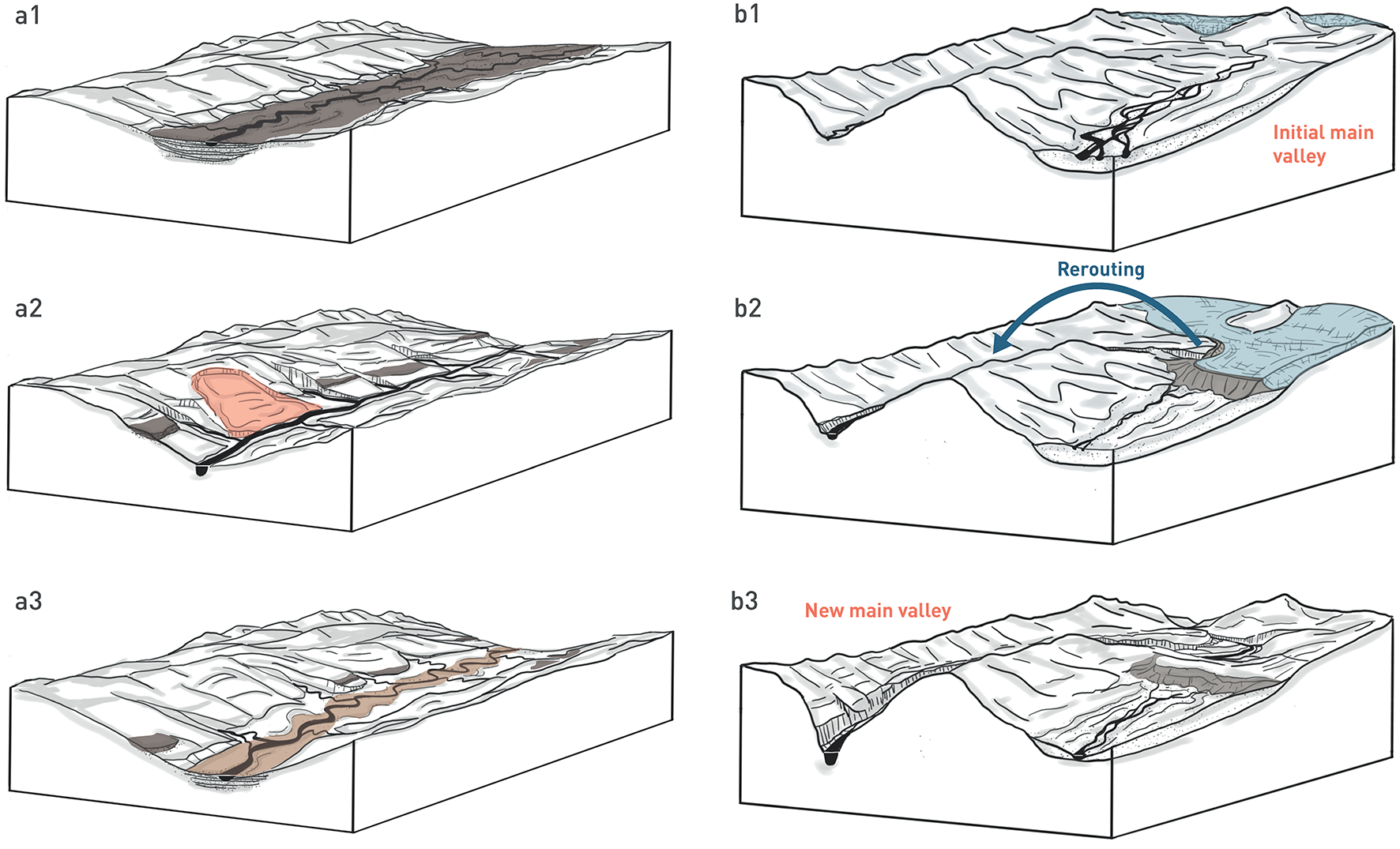
Fig. 6‑22:Conceptual figures of local landscape evolution by (a) local baselevel fall of a main river, and (b) the formation of a breakthrough channel in an ice-marginal setting

Sequence (a) starts with a mature main river valley characterised by a wide aggraded valley floor (a1; dark brown). A pulse of fluvial incision of the main river through the former valley infill and into the bedrock (local baselevel fall) follows in (a2). This stage includes the formation of terrace relicts above the former valley floor (dark brown), propagation of the incision signal along tributary streams and hillslope response (e.g. landslides; red). More advanced adjustment to the new local baselevel is indicated in (a3), with the formation of a new main valley floor (light brown) and a general widening of the valley shape by continuing local erosion. Sequence (b) starts with a pro-glacial main valley (b1; glacier shown in light blue). Glacial advance in (b2) causes blocking of the former main valley by a terminal moraine (greyish brown), and subsequent rerouting of the ice-marginal main drainage into an adjacent valley. The new drainage erodes the former ridge at the location of overspill, thereby creating a breakthrough channel that evolves to a new main river valley after glacial retreat (b3).

Local topography in the greater Bözberg area of Northern Switzerland – a qualitative and quantitative comparison with the Wutach area of the Swabian Alb

The majority of the terrain in Northern Switzerland is characterised by a low-relief cuesta land­scape (see Fig. 6‑23a as an example). Wide fluvial channels and extended terrace systems define the postglacial terrain of Northern Switzerland. While both Höhere and Tiefere Deckenschotter deposits are preserved in isolated relicts, the Hochterrasse and Niederterrasse deposits follow a continuous and traceable fluvial network (Fig. 6‑20). However, deviations from these general patterns of a distinct long-lived fluvial network exist at various scales. Small-scale lateral channels (breakthrough channels), for instance, are observed throughout Northern Switzerland. Evidence exists for temporary features (e.g. Wangetel between Jestetten and Wilchingen or Herblingertal between Thayngen and Schaffhausen) or persistent channels (e.g. Rhine Valley between Rüdlingen and Tössegg). Most of these channels developed in association with large foreland glaciations, either by glacial or postglacial impoundment of a present drainage and sub­sequent overspill or by ice-marginal drainage (compare Fig. 6‑22b; e.g. Keller & Krayss 2000). Such local changes in the drainage can have a profound influence on the adjusting landscape.

Holocene geomorphological process rates (e.g. shallow landsliding, overall denudation processes) in the Bözberg area of the JO siting region seem low based on a morphological landscape assess­ment (Fig. 6‑23a and c; Ludwig 2018). Present-day terrain elevation within the extended study area ranges from around 700 m a.s.l. at the highest hilltops of the External Jura (Schinberg, Geiss­berg) to 300 m a.s.l. at the outlet of the Sissle River into the Rhine. Given this comparably high local relief, hillslope processes play a relevant role in shaping the landscape of the JO siting region and its surrounding areas. For instance, historical landslides from the study area have been docu­mented by Baltzer (1876), Hartmann (1928, 1950) and Haefeli (1940). Fig. 6‑23 shows that, in general, the central part of the siting region appears "quiet" with respect to landsliding. A large proportion of this region consists of the "upland low-relief area" of the "Bözbergplateau" and "presumably unfailed hillslopes", associated with the lithostratigraphic domains of Tertiary sedi­ments (Molasse), Villigen Formation and Wildegg Formation (compare Fig. 6‑21). On the other hand, landslides within the mapping area appear to be clustered within Tertiary sediments (Molasse) along the Aare River, i.e. the southern margin of the Bözbergplateau (southeastern corner of the siting region) and within various lithostratigraphic units along the Mandach Thrust north of the siting region, from Frickberg in the west to Böttstein next to the Aare in the east (Fig. 6‑23c).

A prominent example of a larger-scale landscape adjustment to drainage changes is represented by the Wutach Gorge in the Swabian Alb (Fig. 6‑23b and d), where a stream capture by a tributary of the Rhine River some 18 kyr ago has caused a significant baselevel drop (Einsele & Ricken 1995, Hebestreit 1995). From its headwaters at Feldberg (the highest elevation of the Black Forest, 1'493 m a.s.l.), the Wutach approximately flows in an east direction until reaching the location of the Late Pleistocene stream deflection near the village of Achdorf. Prior to drainage reorganisation, the former Donau-Wutach¹⁶ here continued its eastward course along the present-day Aitrach Valley (Fig. 6‑23d) towards the Danube. This changed when the Donau-Wutach was captured by the Rhine Basin from the south, as a result of headward erosion by a pre-existing Rhine tributary, referred to as the Rhine-Wutach.

Alternatively, coeval aggradation by the former Donau-Wutach leading to an overflow across the drainage divide has been presented as an additional explanation for the stream deflection, at least as a final trigger mechanism (Hebestreit 1995). Such aggradation may have been favoured by glacially enhanced sediment flux from the former Feldberg Glacier that occupied the Donau-Wutach headwater region during the last glaciation. As determined by the course of the former Rhine-Wutach, the present-day Wutach is directed to the south / southwest at Achdorf (Fig. 6‑23d), until finally joining the Rhine to the south at an elevation of ~ 315 m a.s.l. This elevation of the Rhine corresponds to a much lower local erosion base than was set by the Danube prior to drainage reorganisation.

The adjustment of the drainage system to this lower local baselevel is expressed by the remarkable incision of the Wutach stream, which reached its present-day level by an incision of up to 150 m within only 6 kyr (Einsele & Ricken 1995). Both upstream and downstream from this point, the incision of the Wutach has produced deep valleys and gorges in the present-day landscape. The adjustment of local topography to the local baselevel fall is further expressed by an attenuated, but still ongoing hillslope response by landsliding along these incised valleys (Fig. 6‑23b, d).

In the following paragraphs, the transient landscape around the Wutach gorge and the neigh­bouring Randen area is briefly compared with the landscape of the Bözberg (JO siting region) using denudation and chemical weathering rates based on cosmogenic radionuclides (¹⁰Be, ³⁶Cl), alongside weathering rates from stream water chemistry (Fig. 6‑23e and f for a simplified syn­thesis). Both areas share a comparable stratigraphy, with alternations of slightly inclined erosion-resistant (e.g. limestones) and more easily erodible units. A total of 26 samples of ³⁶Cl and 11 samples of ¹¹Be concentrations for catchment-average and hillslope¹⁷ denudation rates in calcite and quartz were measured, respectively. More information on the method and sampled sub-catchments are provided in Nagra (2024k).

Catchment-wide denudation rates indicate the lowest rates in the low-relief areas of the Bözbergplateau and the incised carbonate valleys of the Randen area (0.05 – 0.1 mm/yr), similar to that described earlier by analogy with surrounding areas (Schnellmann et al. 2014). In these areas, weathering accounts for ~ 75% and 50% of the denudation, respectively (based on measure­ments of denudation and weathering rates outlined in paragraph above). Along the flanks of the Bözbergplateau, where hillslope channel processes are more active, these rates double and are within the range of long-term incision of the Rhine and Aare (Fig. 6‑23e). Erosion and weathering each contribute ~ 50%. Highest rates (0.3 – 0.5 mm/yr with < 20% weathering) were measured in the rapidly incising Wutach gorge upstream of the capture point (Fig. 6‑23f). Such high rates reflect adjustments to the transient process of the upper Wutach catchment capture but will reduce with increasing maturity of the landscape, as observed in the neighbouring Randen area.

Combined, the data show that, in areas of low relief (e.g. Bözbergplateau), weathering dominates over physical erosion. In areas of intermediate slopes (Randen, Bözberg flanks), the amounts of erosion and weathering are similar. In contrast, the rapidly incising upper Wutach is dominated by pronounced physical erosion processes.

These new quantitative data confirm the range of previously reported intermediate-term denuda­tion rates from the North Alpine Foreland (usually below 0.3 mm/yr) or adjacent regions, such as the Black Forest (~ 0.01 – 0.1 mm/yr), which are also based on catchment-wide denudation rates, measured using cosmogenic nuclides (see Schnellmann et al. 2014 and Nagra 2024k for a summary). It is concluded that, on average, intermediate-term denudation rates below 0.1 mm/yr can be expected in the area of the siting regions. In the case of future modulation of the drainage system with baselevel drop or if exposure of different rock types leads to increased local relief, these rates can multiply locally but for a limited period in time.

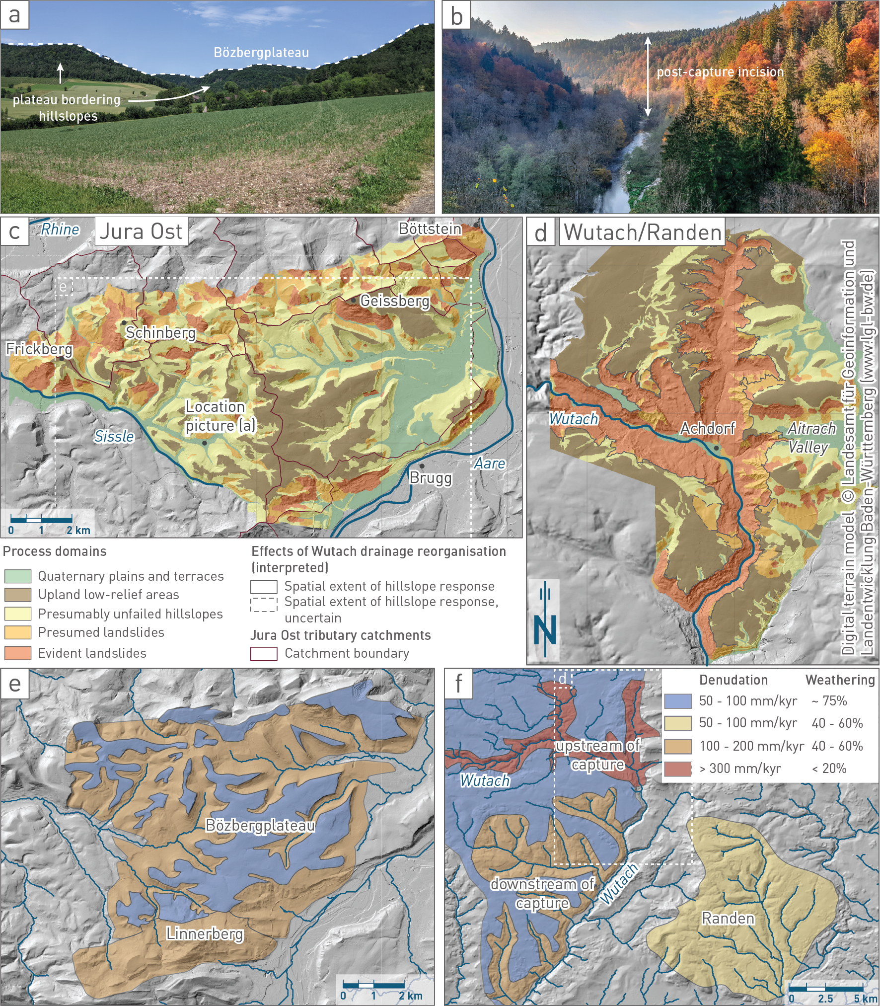
Fig. 6‑23:Comparison of a geomorphically quiet (JO) with a highly active landscape (Wutach)

Comparison of the study areas. (a) Field picture of a valley carved into the Bözbergplateau. Note the relatively straight mountain tops of the plateau. (b) Field picture of the narrow Wutach gorge cut into Muschelkalk carbonates after the river capture event ~ 18'000 years ago. (c) Map of (hillslope) process domains for the JO study area (Ludwig 2018; see details there for definition and criteria of individual process classes). (d) Map of (hillslope) process domains for the Wutach catchment around Achdorf (digital elevation model: LGL 2010). (e) Simplified synthesis of interpreted denudation rates based on basin-wide and hillslope sampling of cosmogenic nuclides of the Bözberg area. (f) Interpreted denudation rates of the Wutach and Randen area. The colours also indicate the approximate percentage of weathering contributing to the total denudation rate (Fig. 6‑23a, b, e, and f are courtesy of R. Ott, see also Nagra 2024k).

Glacially overdeepened, often back-filled troughs in Northern Switzerland are distinct features that have been eroded below the local erosion base. Areas with vestiges of deep glacial erosion constitute the third important reference compartment (see Section 6.4.1.1) for the erosion assessment.

Main glacial and subglacial erosion processes

The main processes of direct glacial erosion are abrasion and quarrying, which depend on the temperature and velocity of the basal ice, debris concentrations, bedrock properties, ice thickness and subglacial water pressure (e.g. Iverson 2002, Bennett & Glasser 2009, Burki 2009, Swift et al. 2015). Significant wear to the glacier bed can also be caused by subglacial fluvial action, similar to the bedrock incision by subaerial streams. The efficiency of subglacial drainage not only affects meltwater erosion but also likely plays a predominant role in evacuating sediments produced by erosion and thus keeping bed surfaces accessible for further erosion. Concerning integrated effects over large areas, abrasion and quarrying may be largely responsible for the overall eroded volumes (e.g. Drewry 1986, Burki 2009). However, with respect to maximum possible erosion depths, subglacial fluvial action likely plays an important role (Fischer & Haeberli 2010).

The latter view is supported by climate-driven ice-flow modelling (see Section 6.3.2, Fig. 6‑16). Transient ice-flow modelling of the Rhine Glacier system over the course of the last glacial cycle indicates that the sliding distance is greatest at the base of Alpine valleys where sliding is fastest, and the duration of ice occupation is longest (Fig. 6‑16c). However, the sliding distance does not correlate well with the location of existing overdeepenings in the Alpine Foreland owing to the smaller sliding speeds near the ice margin and the short time period during which ice covered the distal foreland (Fischer et al. 2021). On the other hand, time-integration of the flow accumulation area yields a metric for erosion by subglacial water flow. Results from simulations of the Rhine Glacier system during advance and retreat in the foreland indicate that subglacial water discharge is high and focused along glacial valleys and existing overdeepenings (Fig. 6‑16Fig. 6‑30d).

The formation of glacial overdeepenings is likely the result of the combined action of ice and basal water flow and depends on the extent to which processes and feedbacks are able to focus erosion and maintain the evacuation of water and sediment (Cook & Swift 2012). The deeply incised troughs and overdeepened valleys in the Swiss Plateau therefore presumably formed time-transgressively during periods of ice advance, when the steep surface slope of the ice margin provided the large hydraulic gradients necessary for a vigorous subglacial water flow and an efficient sediment evacuation from the ice-bed interface. They may also have formed during the retreat phase by the outburst of subglacial meltwater dammed behind a cold-based ice margin or a marginal permafrost wedge (Piotrowski 1994, Hooke & Jennings 2006, Stumm 2010, Kehew et al. 2012, van der Vegt et al. 2012).

Deep glacial erosion is expected to slow down within more erosion-resistant rocks (such as limestone). Good examples for such behaviour are observations from the lower Aare Valley (Fig. 6‑25), but also from the Finger Lakes in New York (e.g. Mullins et al. 1996). The Cayuga Lake Basin, for instance, seemingly shows a limiting effect on incision when reaching the Ono­daga limestone (Mullins et al. 1996, Bloom 2018, see also Nagra 2024k for more detail). When space is available, subglacial erosion tends to widen the overdeepening within the softer material instead of vertically incising into the harder rocks. In contrast, inneralpine overdeepenings carved in harder-to-erode rocks can reach a significant depth (e.g. Magrani et al. 2020). Here, however, topographic steering inside the preconditioned Alpine valleys may dominate over lithological control. Limited efficiency of erosion in limestone might also be the case, for example, because large amounts of subglacial water may be lost into the underlying limestone karst if available (a process known as underdraining; Grust 2004, Gremaud & Goldscheider 2010, Braakhekke et al. 2017) thereby preventing the build-up of high water pressures that are favourable for active erosion, and the energetic water flow necessary for sediment evacuation.

Sills within the overdeepenings may locally lead to the formation of narrow inner gorges/canyons (e.g. Bandou et al. 2023) but very limited data is available about the abundance of such features in the distal Alpine Foreland.

Glacial overdeepenings in Northern Switzerland

The glaciations in Northern Switzerland caused deep erosion into the bedrock (mainly Molasse, but in the Aare Valley lime- and marlstone were also affected) and the formation of overdeepened troughs (Fig. 6‑24). The glacially eroded Molasse assemblage in Northern Switzerland comprises a variety of different, yet mostly easily erodible, rock types. On the rare occasion where over­deepening in Northern Switzerland reached limestone (Fig. 6‑25), the depth is considerably reduced. Furthermore, visual inspection of the map pattern (Fig. 6‑24, east of Aarau and south of Brugg) suggests that overdeepening tends to widen within the easier erodible Molasse assemblage rather than to extend into the harder limestone units. Although a multitude of reasons could be considered for this effect (e.g. distance to ice margin, topography of Internal Jura as a barrier), lithological control seems reasonable (see Section 6.4.3.3 for more detail).

Some of the troughs in Northern Switzerland, such as the Strassberg Trough (Fig. 6‑26b), show a multiphase filling, whereas the fillings of others seem to be dominated by only one phase (e.g. Gebenstorf – Stilli Trough, Fig. 6‑25, Fig. 6‑26a; Gegg et al. 2021). There is evidence for a multiple reactivation of the same trough by several glaciations (e.g. Bodensee Trough, Strassberg Trough), but in other cases troughs can occur side by side (e.g. Strassberg and Bülach Troughs, Fig. 6‑26b), indicating a temporal and lateral shift of the overdeepening process.

The finding of pre-LGM sediments preserved within many overdeepenings (e.g. Dehnert et al. 2012, Buechi et al. 2018) suggests that not all glaciations were able to excavate the postglacial sediment infill of the previous glaciation and cause renewed overdeepening (Buechi et al. 2018). In ice-marginal areas of the North Alpine Foreland this preservation is often a result of changes in spatial focus and magnitude of subglacial erosion between different glacial periods (Buechi et al. 2024). On the other hand, progressive deepening over successive glacial cycles may also have taken place because ice flow is likely to be diverted from hills and ridges into already existing troughs and valleys (Kessler et al. 2008). This topographic steering is part of a positive feedback mechanism that causes the thicker and faster-flowing ice to generate more basal melting, which in turn will further increase basal sliding and sediment evacuation and consequently result in enhanced erosion. The glacial overdeepenings in the foreland often show a system of branching troughs (e.g. in eastern NL and ZNO, see Fig. 6‑24). Breakthrough channels or ice-marginal drainage (Fig. 6‑22b) can lead to new passages for ice that might subsequently focus (sub)glacial erosion with overdeepening. This process is thought to be more likely with repeated glaciations.

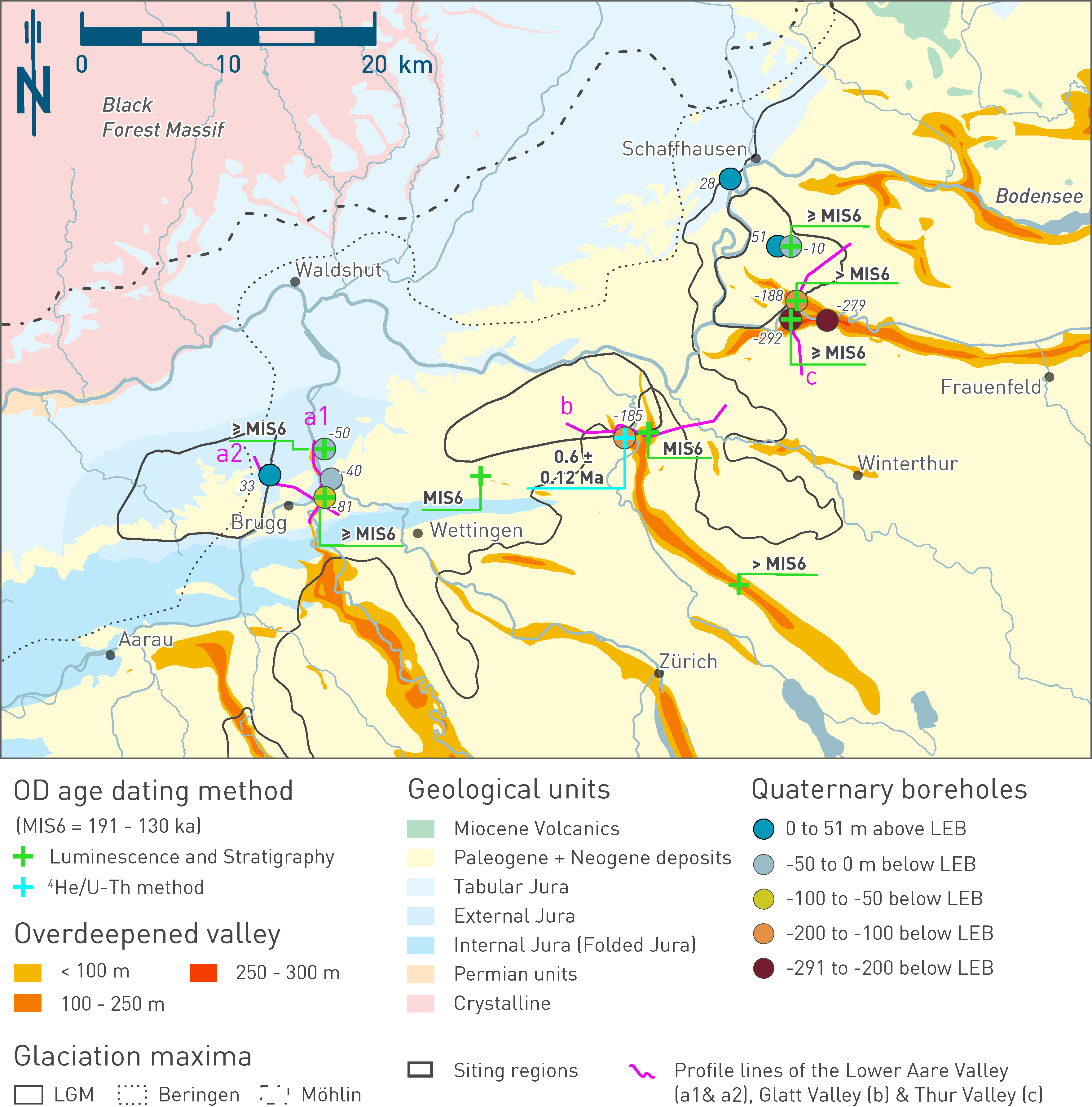
Fig. 6‑24:Overview map showing the glacial overdeepenings and the underlying rock units

Overdeepening depth is depicted by sediment thickness below the local erosion base. The LGM (Bini et al. 2009) and the Beringen and Möhlin ice extents (Preusser et al. 2011) are drawn as solid, dotted and dash dotted black lines, respectively. It is conspicuous that almost exclusively the more easily erodible Molasse sediments were overdeepened (yellow colours). An exception is the lower Aare Valley, east of the JO siting region, where, amongst others, erosion-resistant Malm limestones were glacially overdeepened (Fig. 6‑25). The locations of boreholes drilled during Nagra’s Quaternary investigation programme are colour-coded and labelled with respect to their depth below the local erosion base. Selected ages reveal the timing of filling and thus postdate the deep glacial erosion event (e.g. Tomonaga et al. 2024, Mueller et al. 2024, Gegg et al. 2021). Also shown are the locations of the four interpretative cross-sections (a) through and across the lower Aare Valley, (b) across the Glatt Valley, and (c) across the Thur Valley which are shown in Fig. 6‑25 (a1) and Fig. 6‑26 (a2, b and c).

It is not always clear whether the observed multiphase backfilling cycles represent single advances within one glacial or different glacial stages. In general, the glacial sediments of over­deepened troughs are difficult to date, and available ages have large uncertainties. Evidence for significant overdeepening in Northern Switzerland exists for the Beringen and Möhlin glaciations. The oldest age so far, derived for the older part of the filling of the Strassberg trough, revealed a minimum age of 610 ± 120 ka applying the ⁴He/U-Th dating method on porewaters (see Nagra 2024k, Tomonaga et al. 2024 ). Few glacial troughs are known to have been eroded into the bedrock during the LGM, although at positions closer to the Alpine chain (e.g. perialpine lakes). In contrast, mostly inlaid terminal glacial overdeepenings were formed in the distal foreland (Buechi et al. 2024). However, the Habsburg glaciation was of similar glacial extent and may be responsible for overdeepening in the study area such as the Birrfeld Trough. Dating efforts accompanying Nagra’s Quaternary drilling programme are summarised and discussed in Nagra (2024k).

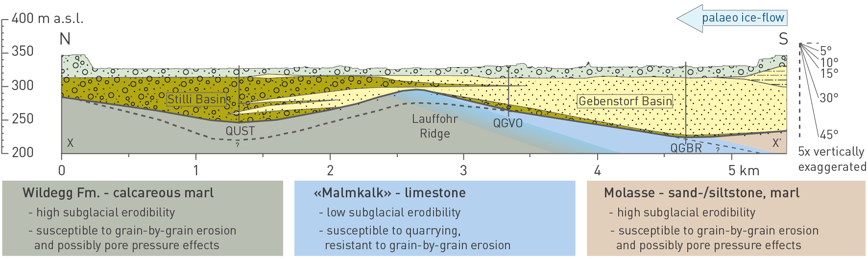
Fig. 6‑25:Longitudinal profile through the Gebenstorf – Stilli Trough close to Brugg

The section (see Fig. 6‑24; a1) is based on seismic cross-sections and boreholes (Gegg et al. 2021) . The orientation of the profile and relative amounts of erosion indicate that the Malm limestone forms a resistant zone in which the overdeepening capacity decreases relative to the Molasse to the south and calcareous marls to the north.

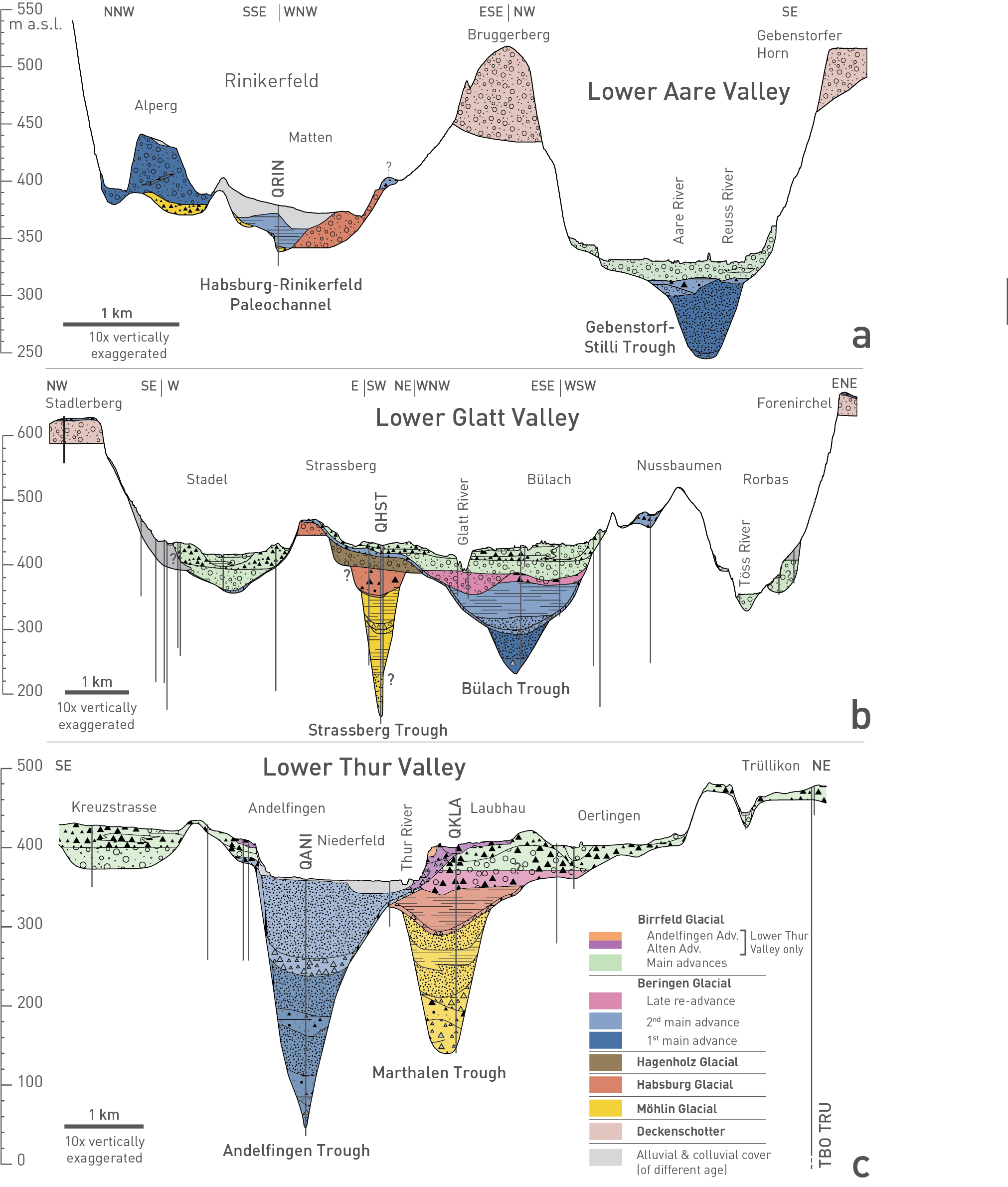
Fig. 6‑26:Cross-sections characterising the Quaternary deposits in the lower Aare Valley, the Glatt Valley and the Thur Valley

The sections represent an integrated interpretation of high resolution 2D seismic data, bore­hole and outcrop data (Nagra 2018). The 10× vertically exaggerated profiles highlight forms, depths and filling of selected and representative glacial overdeepenings. (a) Lower Aare Valley with the fluvioglacial Habsburg – Rinikerfeld Palaeochannel (QRIN) and over­deepened Gebenstorf – Stilli Trough (after Gegg et al. 2021). (b) Glatt Valley with the overdeepened Strassberg (QHST) and Bülach Troughs. (c) Lower Thur Valley with the overdeepened Andelfingen (QANI) and Marthalen (QKLA) Troughs (Buechi et al. 2024). See Fig. 6‑24 for location.

In this section, the concept of landscape compartmentalisation introduced in Section 6.4.1.1 and the erosion history highlighted in Sections 6.4.1.2 to 6.4.1.4 are used to derive a brief summary of the present landscape and to interpret the main differences between the three siting regions (Section 6.4.2.1). Combined with the respective repository depths, these differences provide site-specific constraints (Section 6.4.2.2) for the erosion assessment. Section 6.4.2.3 provides a brief introduction to the model cascade and the specific approach, including an introduction to the methodology of structured expert elicitation, to incorporate uncertainties in the assessment of future erosion. This assessment forms the basis for evaluating future erosion processes (Section 6.4.3), with the focus on the evolution of repository overburden thickness. Results are presented in Section 6.4.4.

In Sections 6.4.1.2 to 6.4.1.4, it has been shown that the Quaternary landscape of Northern Switzerland is shaped by the effect of multiple glacial/interglacial cycles with phases of sediment accumulation and vertical incision (including multiphase deep glacial erosion). The distance from the Alpine chain and from the ice margins, as well as the erodibility of the outcropping rocks led to marked differences between the present-day landscapes of the three siting regions. These differences are highlighted along the summary profile through all the siting regions (Fig. 6‑27). The consequences which these differences have with respect to the siting regions (e.g. depth of the Opalinus Clay) and which thus define the different boundary conditions are further described in the following Section 6.4.2.2.

Mainly because of the general SSE-ward dip of the strata in Northern Switzerland different lithologies crop out in the three siting regions, i.e. mainly Mesozoic rocks in JO and Paleogene/ Neogene rocks in NL and ZNO. The bedrock underlying Quaternary unconsolidated sediments in NL and ZNO, i.e. the rocks that are subject to erosion, are comprised of easy-to-erode assemblages of Molasse sediments of Northern Switzerland. Harder-to-erode rocks (e.g. Malm limestone) are located only at depths of several hundreds of metres. JO, in comparison, is characterised by a cuesta landscape with alternating harder- and easier-to-erode rocks (Fig. 6‑21). Harder rock types (see Fig. 6‑27) are presently located close to the surface and probably influenced the present stability of the plateau-like landscape in JO.

No glacial overdeepening is located within the HLW perimeter of JO; the closest occurrences can be found in the lower Aare Valley east of JO. In contrast, in the NL and ZNO siting regions, glacial overdeepenings are significantly deeper than in the lower Aare Valley. This observation can be attributed to two factors. On the one hand, the glacial troughs in NL and ZNO were cut into more erodible sedimentary rocks of the Molasse (Fig. 6‑24), while the hard limestone layers in the lower Aare Valley slowed down erosion (Fig. 6‑25). On the other hand, glaciations during past ice ages have impacted the three siting regions to varying degrees. The map of the ice extent shown in Fig. 6‑18d, Fig. 6‑24 and the simplified bars in Fig. 6‑27 illustrate these differences based on three extensive and relatively well-known glacials in Northern Switzerland (Möhlin, Beringen and Birrfeld). Only the most extensive glaciations reached the JO siting region, and the glaciers were presumably less thick than in NL and ZNO. During the last ice age, the ice cover in ZNO was thicker and more extensive than in NL. Such patterns can be expected during future glaciations.

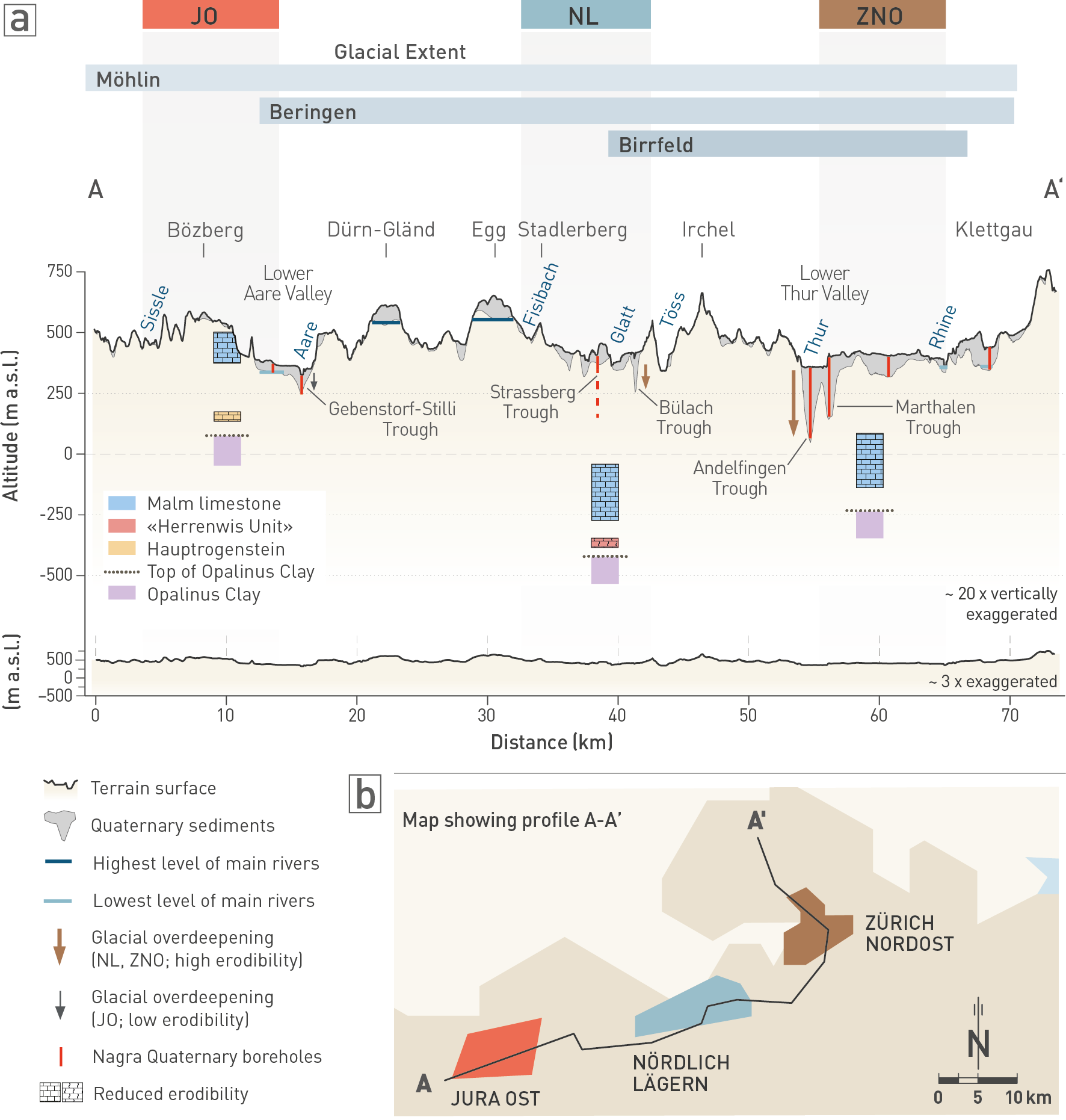
Fig. 6‑27:Cross-section through the siting regions with the morphological and geological conditions that are key to assessing future erosion processes

The synthesis cross-section (a) shows the present-day topography, the main palaeoriver levels (highest fluvial level in dark blue and lowest level in light blue, the latter corresponds to the LEB) and glacial overdeepenings. Quaternary boreholes drilled during Nagra’s investi­gation programme are shown (Strassberg Trough borehole dashed because it is not located at the cross-section position, see Fig. 6‑26b for comparison), as well as a simplified stratigraphy focusing on the host rock (Opalinus Clay) and erosion-resistant rock types above it (Fig. 6‑21). The blue bars above the figure show comparatively well-known extents of earlier glaciations (Fig. 6‑18d). The extent of the Birrfeld glaciation marks the LGM of the most recent ice age around 21'000 years ago. The Beringen and Möhlin glaciations formed during earlier ice ages that probably occurred between 100'000 and 650'000 years ago (Fig. 6‑12). (b) Simplified map showing the location of the cross-section with respect to the siting regions.

The differences illustrated above (e.g. occurrence of glacial overdeepenings or local topography) become effective when considering the depth-dependent barrier function (Sections 6.1.2, 6.5.2.2) of the host rock and potentially relevant tectonic- and climatic-driven surface processes. Fig. 6‑28 exemplifies this effect by showing the fractions of the different landscape elements (compart­ments) with respect to the depth of the Top Opalinus Clay (i.e. the repository host rock) for each siting region. These fractions are shown for (1) the entire HLW siting regions, (2) the provisional disposal area (reflects the ~ 1 km² outline of the repository project for high-level waste; for location see Fig. 6‑34) and (3) the provisional disposal area including spatial reserves (see Nagra 2024e for further information). Note that the final calculations of the erosion assessment refer to the provisional disposal areas.

The depth of the provisional disposal area (approximately 50 m below the Top Opalinus Clay; see Fig. 6‑28, brown boxes) with respect to the local erosion base is deepest in NL (794 m at centre, 764 m at most shallow location), and considerably less deep in JO (291 m at centre, 270 m at most shallow location). On the other hand, the amount of local topography is significantly larger, both as median (206 m) and as range, in JO than in NL (median 113 m) or ZNO (median 84 m, red boxes). This local topography adds additional overburden thickness above the reposi­tory needed to maintain the barrier effect (Section 6.1.2).

The distribution of glacial overdeepenings in the siting regions varies significantly. As already highlighted above, no overdeepening is observed in the entire HLW siting region of JO. The box plots for glacial overdeepenings in NL and ZNO (blue boxes in Fig. 6‑28) not only show the occurrence of such feature in the siting regions or the spatial reserves but also show that they can be very deep (> 150 m below local erosion base [LEB] in the entire HLW areas of NL and ZNO); more often or in larger parts, however, they do not reach more than about 70 m below LEB with median values around 30 m. This is an important observation when addressing this effect in the future assessment.

Accordingly, to compare the three sites with their different boundary conditions in an unbiased way, the landscape compartmentalisation into local erosion base, local topography, and glacial overdeepenings was transformed into a model cascade (see next section).

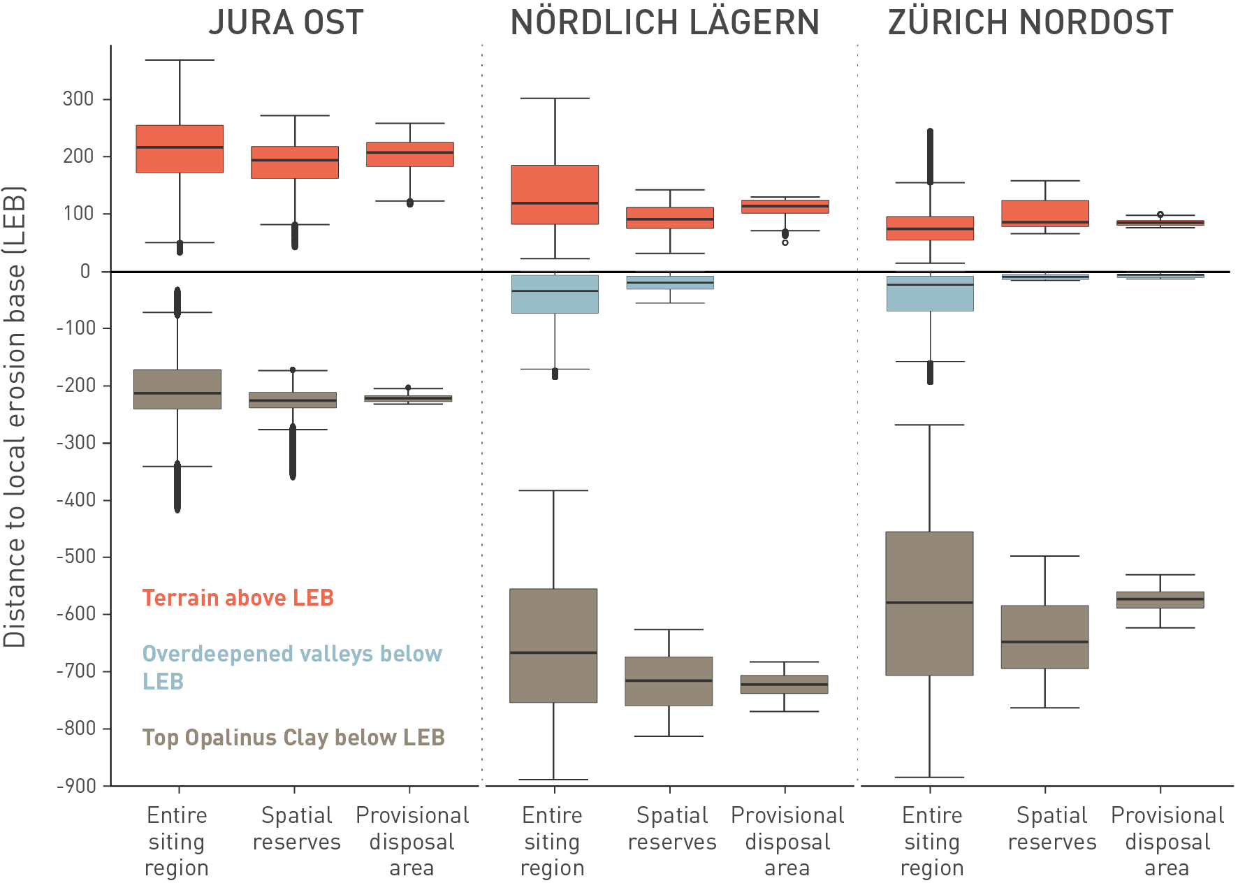
Fig. 6‑28:Site-specific constraints of the landscape compartments within the siting regions

Depth profiles showing boxplot statistics on the main compartments with respect to the local erosion base (0 m line). Boxes entail the interquartile range between 25^th – 75^th quantiles, the whiskers the extreme values, as derived from multiplying the interquartile by 1.5. Values outside the whiskers are considered statistical outliers. The siting regions share different portions of the landscape compartments. The depth of the provisional disposal area with respect to the local erosion base (LEB) is deepest in NL, and considerably less deep in JO. On the other hand, JO is covered by significant terrain above the LEB (local topography) and this site is less affected by glaciations. JO has no overdeepened area within the siting region.

For the calculation of the difference raster LEB – Top Opalinus Clay, raster datasets of the LEB (Pietsch & Jordan 2014) and the horizon Top Opalinus Clay (Nagra 2014b) were used. In comparison to the local model Top Opalinus Clay of 2014 (Nagra 2014b), the more recent 3D horizon model of the sites (Nagra 2024m), covering the zones of the spatial reserves and the provisional disposal areas, shows the following average differences: 18 m deeper in JO, 12 m deeper in NL, 6 m shallower in ZNO. Note that the assessment of future erosion presented in Section 6.4.3 is based on the recent 3D horizon model documented in Nagra (2024m).

Managing knowledge and uncertainties in the context of assessing the long-term safety of a deep geological repository is challenging, in particular because of the long time span to be considered. In this section, the main procedure used is highlighted.

The model cascade

Two main questions are addressed to ensure barrier integrity and long-term safety with respect to future erosion: (i) how much remaining overburden thickness is expected in the siting regions after the periods under consideration and (ii) what is the probability of excavation at the end of one million years? Accordingly, the data provided here are used for the safety-based comparison of the siting regions and as input for safety analysis. The remaining overburden in metres and excavation probability in percent are the main outputs of the erosion model (Fig. 6‑29). Both outputs can be calculated for any position within the area of interest. The focus is on the location of the provisional disposal area and its anticipated depth within the host rock Opalinus Clay.

The structure of the erosion model resembles a "Roman Fountain" where the output of Model A (Fluvial incision, i.e. future evolution of the local erosion base) generates input for Model B (Evolution of local topography) and Model C (Deep glacial erosion). The separate consideration of each of the three processes and subsequent combination in the model cascade allow future erosion in the siting regions to be critically assessed and compared.

Model A starts with simulations of the fluvial incision along the Hochrhein. Model B incorporates the 3D geology and simulates the response of local rivers and hillslopes to the derived incision of Model A, extracted at three selected points downstream of each siting region (Section 6.4.3.1). Both stable drainage networks and plausible alternative drainage scenarios (Section 6.4.3.2) are included to account for uncertainties in future channel dynamics, especially in JO. The latter considers the development of new valleys cutting across topographic highs, such as the Bözberg­plateau, in conjunction with large future foreland glaciations. Output of Model B provides the remaining overburden thickness and an excavation probability with excluding glacial over­deepening. Incision of Model A and the different drainage scenarios of Model B are input data for Model C. The calculation chain of Model C (Section 6.4.3.3) combines several aspects to be evaluated with respect to future deep glacially eroded troughs. The output of Model C provides estimates of remaining overburden thickness and excavation probabilities including glacial overdeepening.

To consider uncertainties for timescales of 100'000 and one million years, a hybrid approach was developed with as much probabilistic treatment as possible. Where a probabilistic treatment was not feasible, scenarios were specified covering what was considered a critical range of possibilities. The whole process was guided by a sensitivity analysis to identify critical parameters and processes in the model cascade. Models A and B are based on numerical simulation, while Model C processes the uncertainties analytically.

Expert elicitation

In the context of future erosion modelling, like in many other areas of science and engineering, modelling has to be carried out against a background of pronounced uncertainties. Whenever there is not enough observational data to determine these uncertainties quantitatively, it is unavoidable to employ expert knowledge for this purpose (Oppenheimer et al. 2016). Within the solid-earth-geosciences, this is particularly the case for seismic and volcanic hazard and risk assessments, in particular when nuclear facilities are involved. However, more recently, expert elicitation has been used in assessment of climate parameters and models (e.g. Yucca Mountains; Dewispelare et al. 1995, Sebok et al. 2022, Bamber et al. 2019) or even in upcoming topics as carbon capture and sequestration (Moore et al. 2024).

Inclusion of expert knowledge must be carried out in a structured manner, as otherwise the results can easily become unreliable and not reproducible (Budnitz et al. 1997, Oppenheimer et al. 2016). This realisation has led to the development of a number of methodological approaches to structured expert elicitation, of which the protocol of the Senio Seismic Hazard Analysis Committee (or SSHAC; Budnitz et al. 1997) and the Sheffield Elicitation Framework (SHELF; Gosling 2018) are two well-tested examples. The aim of both methods is to describe uncertain quantities of interest (QoI) as probability distributions that represent the expert knowledge of a group, based on expert judgment of their members. It is important to note that there is a certain vocabulary inherent that may be uncommon. To avoid misunderstandings, brief explanations of the most common terms are added below (O’Hagan 2019).

Expert judgement (also expert opinion) describes the individual representation of one (or a group of) expert’s scientific judgement on a specified topic, in this case for instance the uncertainty of a model input parameter. This rational judgement is based on available data and the expert’s scientific know-how and experience and is provided after a training on the influence of cognitive biases (Kahneman et al. 1982) in decision making, especially such as anchoring, availability bias or overconfidence but also the more general aspect of group dynamics.

The probability concept behind expert judgement is that of subjective probability. Subjective probabilities (Cooke 1991) are the expert’s degrees-of-belief formally expressed as probabilities. They are called "subjective" because they follow individual (or group’s) judgements. These pro­babilities are nevertheless informative and scientific (O’Hagan 2019) and one of the existing legitimate probability concepts that meet Kolmogorov’s axioms (Galavotti 2005).

Elicitation describes the process of gaining the expert’s judgement. The uncertainty elicitations for the parameters relevant for the erosion assessment at Nagra followed the SHELF protocol (Gosling 2018), which is a two-step structured group elicitation framework for carrying out the elicitation of subjective probability distributions for quantities of interest (QoI). The actual elicitations are done in workshops which are led by an experienced facilitator (moderator) who has been trained in all aspects of the SHELF protocol.

The first step requires the individual elicitation of a set of quantiles (e.g. median, tertiles/quantiles, upper and lower bounds) for the uncertainty distribution of interest, one for each expert. In the second step, the expert group derives a single group distribution, which reflects an integrated view of the uncertain quantity. This means that all arguments brought up during the group discussions are considered, as they would be seen through the eyes of a rational impartial observer (RIO) (Gosling 2018, O’Hagan 2019) and it requires that all experts exchange their individual judgments with the role of RIO. The RIO perspective takes into account the combined knowledge of the group but gives some (perhaps more convincing) arguments more weight than others. The facili­tator "acts" on behalf of the RIO (and thus in agreement and collaboration with the experts), when aggregating the distributions.

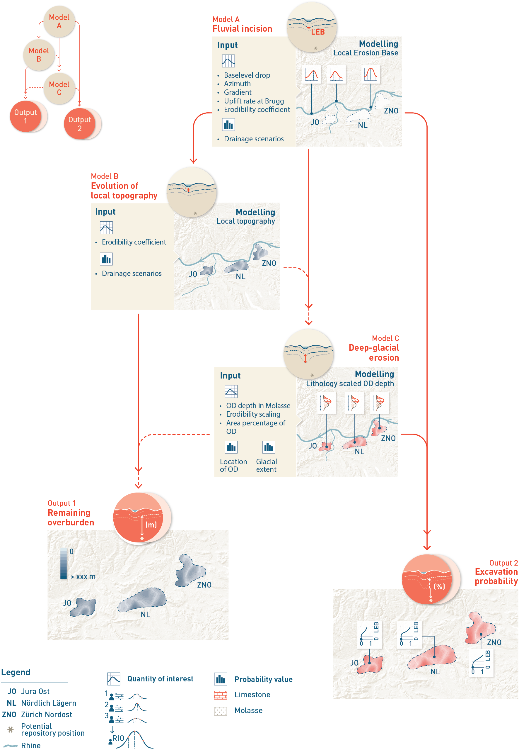
Fig. 6‑29:Simplified flowchart for calculating the remaining overburden thickness and probability of excavation at time T^x

The hybrid probabilistic model consists of three submodels: Model A: simulation of the local erosion base (LEB), Model B: accounting for the effects of local topography, Model C: assessing the probability of glacial overdeepening (OD) and evaluates the combined (glacial and fluvial) probability of incision below a certain vertical position (e.g. the level of the provisional disposal area). Both Model B and Model C depend on the output of Model A. The glacial part of Model C does not depend on the output of Model B. It is based on the LEB and does not account for local topography, i.e. Model C only takes glacial over­deepening events into account that cause an overdeepening below the LEB. However, Model C does depend on scenarios of alternative drainage networks that are developed within/for Model B. Note that final distributions of remaining overburden thickness and excavation probabilities are calculated for selected locations only. Also note that all listed input parameters (left side of subfigures) are quantities of interest for which uncertainties were assessed by elicitation following the SHELF protocol. Finally, it is possible to calculate non-glacial excavation probabilities (parallel to Indicator 1) and combined non-glacial and glacial distributions of remaining overburden thickness (parallel to Indicator 2).

The RIO distributions were fitted with parametric distributions that best reflected the elicited quantile values. Importantly, these RIO distributions comprise the uncertainty that is propagated into the model (Fig. 6‑29). In Fig. 6‑29, all input parameters (left side of each Model) are quanti­ties of interest for which the uncertainties were assessed in SHELF-based elicitation workshops. A total of 34 parameter uncertainties have been evaluated to be used in the modelling or for plau­sibility checks (see Nagra 2024k for more details). Not all quantities, however, were assessed as probability distributions, some were provided as scenario weights or event probabilities. Because the elicitations were conducted within the erosion team at Nagra with usually 3 – 5 experts per workshop, it was particularly important to include both, the expertise in local geology and geomorphology, as well as expertise in process understanding. The facilitator was supported by an external expert with a strong background on statistics and probabilities, who was trained on all SHELF aspects. The high number of parameter uncertainties required prioriti­sation regarding, which parameters to treat with most effort (e.g. a higher number of experts, more time etc.). This prioritisation was supported by a sensitivity study. In exceptional cases, a pragmatic deviation from the protocol was allowed (see Nagra 2024k for more detail).

It is important to recapitulate that a rigorous evaluation of prior and present conditions of the landscape and the processes that shaped it was conducted by an extensive scientific programme over several years. The available outcomes of this programme (see also Nagra 2024k for more detail) were provided to all the experts prior to the workshops to ensure that all experts were 'reading from the same page' and that they had access to the same factual basis. In this report, the main evidence is provided in the previous Sections 6.2, 6.3, 6.4.1, as well as Sections 3.4.5 and 3.5.

In the following sections, RIO distributions are provided for the most important parameters used in the respective models only. They are provided with a brief reasoning, which in turn is based on the evidence provided before, partly supported by additional global data or more process-related expertise, which might then be shown or cited individually. More detail on the modelling and parameters can be found in Nagra (2024k).

Presentation of results

In this report, the results are shown only for the one-million-year timescale, with the exception of the intermediate results of future fluvial incision. The final calculations are provided for the provisional disposal areas of each site. To allow a more qualitative comparison within the wider areas containing the spatial reserves, an abridged calculation was used for a set of additional coordinates (Nagra 2024k) in each siting region. To follow the general procedure of the safety-based site comparison, different outputs were generated to evaluate criterion 2.2 (Erosion) and criterion 3.3 (Predictability of long-term changes) of the Sectoral Plan (SFOE 2008). These out­puts, as well as considerations beyond one million years, are only reported in Nagra (2024k). Of the full range of uncertainties presented by the total assumed probabilities, the 5 – 95% range is considered the "expected range" in this assessment.

In general, it is expected that future erosion processes (both glacial and non-glacial) will be comparable to those prevalent during the Quaternary with a few exceptions:

• The fluvial incision rates are predicted to be lower because the main pulse of incision caused by large-scale drainage reorganisation has diminished (Section 6.4.1.2).

• The most important variations between aggradation and incision periods are expected to be caused by future glacial/interglacial cycles. The long-term incision driven by vertical motion of the rock column will thus be modulated by phases of sediment accumulation with no net vertical incision, comparable Quaternary evolution (Section 6.4.1.2).

• The next glacial inception might be delayed because of the anthropogenic atmospheric CO₂ content (Section 6.3.3).

• The stratigraphic column above the repository sites NL and ZNO contains harder-to-erode rock types (limestones of the Malm) compared to the Molasse, which is currently the outcropping lithology at these sites (Fig. 6‑27, see Sections 6.4.1.4 and 6.4.2.1).

• In addition, further erosional downcutting might decrease the accumulation area of future glaciers, which in turn might result in smaller glacial extents, even with similar climate forcing (Egholm 2022). On the other hand, as a result of the drainage divide shift between Rhine and Danube, the Rhine Glacier might undergo a westward shift with less ice being able to cross the divide and drain towards the Danube (Ellwanger et al. 2011), which in turn might increase the erosion potential in the study area.

For the future erosion assessment, evidence from Quaternary landscape evolution together with process understanding was used to derive probability distributions for the parameters to be applied in the modelling (see Section 6.4.2.3 for a brief overview on expert elicitation). An overview of the main results and associated line of reasoning for each separate erosion process (i.e. model part) is presented in this section. More details are provided in Nagra (2024k).

Future evolution of the local erosion base

The analysis of future fluvial incision of the Hochrhein (i.e. approximately between the cities of between Stein am Rhein and Basel) and thus lowering of the local erosion base is based on the stream power incision model (SPIM) (for more detail see Nagra 2024k). The SPIM is frequently used in landscape evolution models that include tectonic uplift U. The main advantage is the low model complexity and its relatively straightforward numerical implementation, which allows its application to long timescales (10⁵ – 10⁶ years) and to investigate different boundary conditions. According to the SPIM, the rate at which rivers incise is a function of the drainage area A and channel slope S = dz/dx raised to the power exponents m and n, respectively, and multiplied by a bulk parameter K which is a dimensional coefficient of erosion often simply termed erosional efficiency or erodibility coefficient (for more detail see Nagra 2024k).

When addressing the future, it is expected that parameters such as rock uplift U (Section 6.2.2), erodibility coefficient K or upstream drainage area A might change over time. Consequently, the evolution of the intermediate baselevel at the transition from the Alpine Foreland to the Upper Rhine Graben near Basel needs to be considered (Section 6.2.2). These parameters were elicited independently as subjective probabilities (see Fig. 6‑29: Model A, Section 6.4.2.3 and Nagra 2024k).

Rock uplift

Spatial rock uplift is approximated here by a plane, i.e. rock uplift is modelled as a linear function of longitude and latitude. The main assumption is that the Alpine uplift provides the dominant cause for the geometry of the uplift plane. In simplified terms, the main gradient causes higher rates from the external foreland towards the Alps along a direction that is roughly perpendicular to the Alpine chain. However, the plane is based on the uncertain parameters of rock-uplift rate at one position (here Brugg), the gradient at which uplift is rising, and the azimuth direction along which the gradient is applied (see Nagra 2024k for more information). Based on the plane, cal­culated from these elicited parameter distributions, the uplift can be evaluated for any coordinate within the investigated area, for instance, for the locations of the siting regions (Fig. 6‑30, Tab. 6‑1). Note the higher rates for the shorter time frame of 100'000 years that includes similar values as measured using geodetic methods (Section 6.2.2).

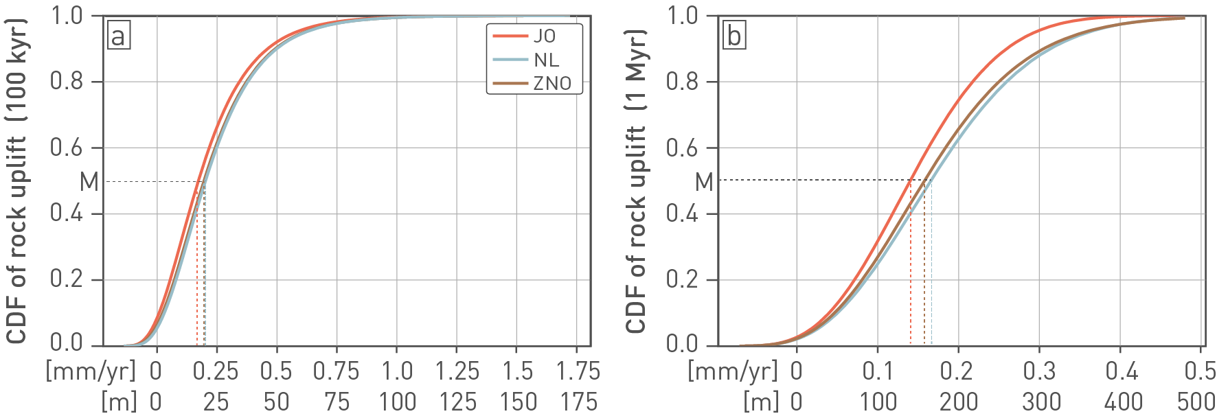
Fig. 6‑30:Inferred future rock uplift rates in the three siting regions over the next 100'000 and one million years

Rock uplift rate is defined as the total rate of bedrock uplift in mm/yr that is expected as a response to tectonic processes and as an isostatic response to loading or unloading, including the response to loss of ice cover. The reference level for rock uplift is the geoid. The estimates are based on the assumption of a planar uplift pattern caused primarily by Alpine uplift. The results are calculated for the location of the provisional disposal areas and shown as cumula­tive distribution function (CDF), where the value of 1.0 (y-axis) equals to 100% cumulative probability. The letter M at both y-scales refers to the median value, i.e. the 50% quantile (value 0.5). The corresponding median values can be read at the x-axes (compare Tab. 6‑1). (a) CDF of estimates for the time frame of 100'000 years. (b) CDF of estimates for one million years. Note that the shorter time frame of 100'000 years allows higher rates (see Nagra 2024k for more details). The lower x-axis translates the rates to cumulative amount of rock uplift for the respective time frames.

Tab. 6‑1:Inferred future rock uplift rates

Rates are estimated at the locations of the provisional disposal areas of the siting regions for 100'000 and one million years, respectively (see Fig. 6‑30). The location of the provisional disposal area is shown in Fig. 6‑34. Values are rounded to the second digit. The 5 – 95% of the total probabilities are considered the expected range in this assessment

Erodibility coefficient

The rock types of Northern Switzerland comprise a variety of assumed resistance against erosion. They were divided into four erodibility classes (EC) based on lithological considerations and the lithostratigraphic units differentiated in the 3D geological model "Nagra Regionalmodell 2012" (Gmünder et al.. The classes comprise EC 1 = Quaternary unconsolidated sediments, EC 2 = Bedrock Class "soft", EC 3 = Bedrock Class "medium", and EC 4 = Bedrock Class "hard" (Fig. 6‑21). It is generally assumed that the classification of erodibility follows the trend of EC 1 > EC 2 > EC 3 > EC 4. This allows distributions to be assigned for the erodibility coefficient (Kvalues) needed for modelling fluvial incision and later local topography (see Section 6.4.3.2) using the SPIM equations.

The geological map of Northern Switzerland 1:100'000 (Isler et al. 1984) was first used to map spatially variable values of the erodibility coefficient K (depending on rock type) on the present-day topography, focusing on the JO siting region and surrounding area (Graf 2022). This first-order assessment was done by extracting ranges of apparent K values from the present-day land­scape based on drainage area and gradient along the channel network. Lithological mapping along the Hochrhein is less distinct than within the 3D geological model. Here, rock types of EC 2 and EC 3 were combined into one class (here ECb) of weak to intermediate resistance to erosion (see Nagra 2024k for more detail).

Importantly, an uplift value of 0.1 mm/yr was spatially uniformly applied to the area used for the K mapping (Graf 2022). Simplified, this means it was assumed that the present-day landscape has evolved under a background rock uplift rate of 0.1 mm/a. Under the chosen SPIM assumption (n = 1, m = 0.45; Nagra 2024k), uplift and K values scale linearly. Accordingly, the elicited distributions for the K values of the four erodibility classes included ranges that were scaled to include variability in the uplift value. These ranges are consistent with the previously elicited one million years RIO distribution for uplift at Brugg (UBR, see above and Nagra 2024k for more detail).

The elicitation followed a rather pragmatic, systematic procedure. First, the general assumption was that the median value of each erodibility class, which was derived by the landscape inversion (Graf 2022), reflects the most robust K value of the respective class. The uncertainty distribution around this value should then reflect the scatter (excluding artefacts originating from low gradients at plateau areas or within flood plains). It should also be accounted for transient effects from spatially non-uniform uplift or incision within the landscape and for the uncertainty caused by the uplift assumption of 0.1 mm/yr (see above).

The mean values of the elicited parameter distributions vary by a factor ~ 1.5 and follow the pattern EC 1 > EC 2 > EC 3 > EC 4. The variability of Kvalues within a distribution can be in the order of one magnitude (see Nagra 2024k).

Baselevel changes

In addition, to account for the downstream change from the tectonic domain of the Alpine Fore­land into the subsiding domain of the Upper Rhine Graben, the parameter baselevel drop (BL) was introduced and elicited (Fig. 6‑31). Baselevel in this context is considered with respect to sea level. Here, negative values reflect net baselevel gain. Accordingly, baselevel gain would mainly correspond to sediment accumulation, while baselevel drop can be both rock subsidence, which is not balanced by sedimentation, or incision into the present Quaternary fill.

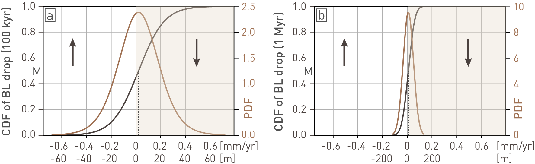
Fig. 6‑31:Total assumed probabilities for baselevel drop downstream of Basel

The total assumed probabilities of the rate of baselevel drop are based on expert judgement (see Nagra 2024k). Probabilities are shown as cumulative distribution function (CDF, see caption of Fig. 6‑30 for explanation) and as probability density function (PDF, brown colour). PDF visualisations allow to assess the most probable values, which are identified by the bulge of the curve (here close to 0 mm/yr). In contrast, lowest probabilities are reflected in the tails (a) 100'000-yr time window and (b) one-million-year time window. Negative values correspond to net baselevel gain. For both time frames, the baselevel downstream of Basel is expected to be stable with a very slight tendency towards baselevel drop. The letter M reflects the median value. The lower x-axis translates the rates to cumulative amount of baselevel change after the respective period under consideration, i.e. 100'000 yr in (a) and one million yr in (b). Note the similar x-axis to highlight the higher rates allowed during shorter periods.

Based on the present-day longitudinal profile and terrace distribution in the Hochrhein and near Basel (Fig. 6‑19 and Fig. 6‑20), the baselevel downstream of Basel is expected to be stable with a very slight tendency towards baselevel drop. However, fluctuations in the order of ~ 30 m (5 – 95%) within the next 100'000 years and up to ~ 60 m gain and ~ 80 m drop (5 – 95%) after one million years appear to be possible in light of the future dynamics of the Upper Rhine Graben and Rhenish Massif (Section 6.2.2) as well as climate-driven sediment flux (Sections 6.3.1 and 6.4.1.2) and were thus included in the uncertainty estimates for future fluvial incision. A baselevel gain of ~ 30 m would roughly reflect the thickness of the Niederterrasse deposits at the location around Basel. Allowing for an additional sediment pulse (e.g. after filling of the Bodensee and Zürichsee), such sediment accumulation seems to be a plausible scenario for a time span of 100'000 years. Yet another plausible scenario would be that, after filling of these peri-Alpine lakes, the sediment pulse fails to appear because of a prolonged interglacial and exhausted sedi­ment sources in the catchments (see Section 6.3.3.1). In such a case, incision into the fill as seen today in large parts of the Hochrhein and Upper Rhine Graben could be expected to continue. Such a scenario could cause net baselevel drop down to the base of the Niederterrasse deposits. Higher fluctuations are allowed in the million-year time window, as it is more likely that larger glaciations will occur (Sections 6.3.3.1 and 6.4.3.3) and supply large amounts of sediment. A baselevel gain of no more than the approximate difference between the top of the Hochterrasse deposits and the river surface and a baselevel drop of approximately half the elevation difference between Bingen and Basel were considered as reasonable assumptions. This estimate is based on the assumption of continued rock uplift of the Rhenish Massif and preservation of the intermediate baselevel near the city of Bingen (see Section 6.2.2).

Changes in drainage area

Based on geometric considerations of the fluvial landscape (Section 6.4.1.2), far-reaching effects influencing the drainage system of Aare and Rhine, similar to those experienced during Pliocene-Quaternary times, are not to be expected at this location for the next million years. A larger piracy scenario that would theoretically be possible late in the period under consideration considers the capture and diversion of the Iller River. Simulations show that such a scenario does not have a major impact on discharge and the vertical erosion potential of the Hochrhein (see Nagra 2024k for more detail). Yet another scenario considers the future increase of the Rhine discharge at the expense of the Danube via karst sinkholes along the Danube. However, even with the full incorporation of the upper Danube catchment into the Rhine catchment, this increase makes only a minor contribution to the fluvial erosion and the longitudinal river profile evolution in the Hochrhein for the next one million years (Nagra 2024k).

Another reasonable scenario would be the diversion and shortcut of the Alpenrhein across a few metre high swell at Sargans, subsequently following a path through the Walensee.

While the Rhine catchment in the area of the siting regions grows at the expense of the Danube, it might lose area towards the Rhone River within the westernmost reaches east of Lac Léman. Headward erosion might capture the Upper Aare, e.g. in the area west of Yverdon (Fig. 6‑19a, see also Nagra 2014c, Dossier III). Such a scenario could cause a baselevel drop with further headward erosion because the Rhone River with ~ 800 km length is significantly shorter than the Rhine River. However, it is not expected that headward erosion would reach the Hochrhein area within the period under consideration. Instead, the loss of Aare catchment would considerably reduce the incision potential of the Hochrhein.

Using a variety of scenarios for changes in future discharge/catchment, as mentioned above (capture of Iller, capture of Upper Danube, diversion of Upper Aare towards west, and diversion of the Alpenrhein across the swell of Sargans) that are ranked by their plausibility, and variants for the parameters based on expert degree of belief, SPIM was used in a Monte Carlo environment to generate probable future river profiles between the outflow of the Bodensee and Basel (i.e. the Hochrhein) at time T^x (100'000 years and one million years) from all parameter combinations (see Nagra 2024k for more detail).

Modelling results

The results are visualised in Fig. 6‑32a for incision after 100'000 years and Fig. 6‑32c for incision after one million years. The left panel shows the realisations of future longitudinal Hochrhein profiles in grey with the present-day river profile (in blue) and the elevations of Bingen and sea level as reference regional baselevels. The darker the future river profiles appear, the more likely is the amount of incision at this position. Baselevel gain flattens the profiles, while baselevel drop allows stronger incision. Because of the more proximal position with respect to the intermediate baselevel in Basel, this influence is largest within the area of JO. The orange boxplots in Fig. 6‑32a and c describe the uncertainty distributions of the rock uplift that the provisional dis­posal areas (circles) might undergo during the same respective time. Using these distributions of rock uplift and future incision, the remaining overburden thickness above the repository location with respect to the local erosion base can be determined (Fig. 6‑32b and d). In these plots, the boxes correspond to specific quantiles (see legend) and the violins reflect the distributions, such that the range of the violins extends past the extreme data points. The bulge corresponds to the most likely values.

The SPIM simulations using all parameter combinations show that fluvial incision itself is not expected to present any threat to the barrier function at ZNO and even less at NL. However, they reveal a considerable number of scenarios in which the repository in JO would be uplifted to, or even above, the future local erosion base (i.e. at the position of the Sissle outlet) after one million years (Fig. 6‑32d). JO would need to rely on the preservation of the additional topography situated above the local erosion base. The results of simulations of the evolution of this local topography are discussed in the next section (Section 6.4.3.2).

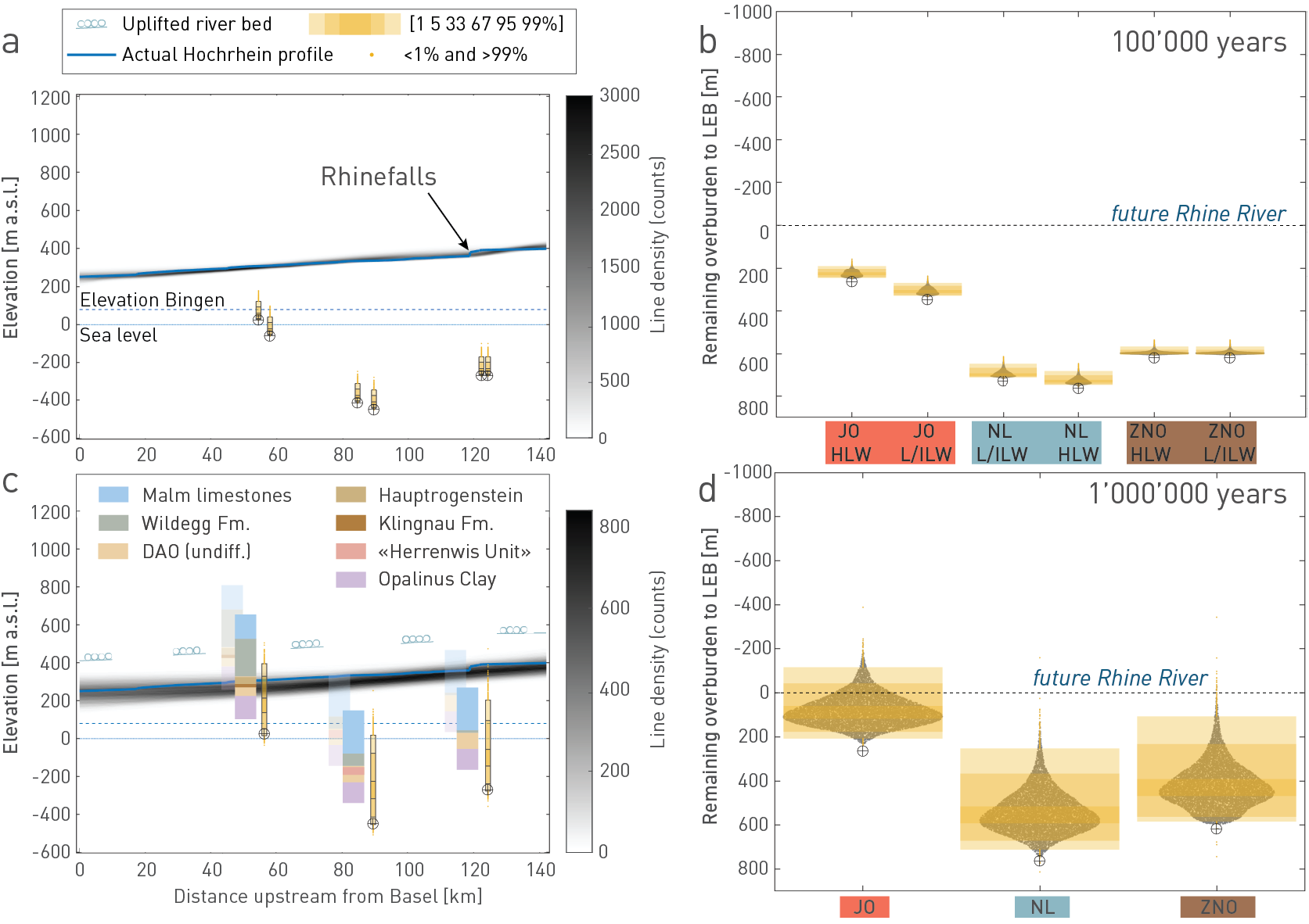
Fig. 6‑32:Results of fluvial incision modelling using the Stream Power Incision Model (SPIM)

The left panel shows the realisations of future longitudinal Hochrhein profiles in grey for 100'000 years (a) and for one million years (c). Also shown are the present-day river profiles (in blue) and the elevations of Bingen and sea level as reference baselevels. The circles correspond to the depth of the provisional disposal areas at the time of emplacement. The orange boxplots above the circles describe the uncertainty distributions of the rock uplift that the disposal areas might undergo in these times. As an example, the stratigraphic columns at the locations of the provisional disposal areas are uplifted according to the median and the 95^th percentile (transparent) – highlighting which units might be incised after one million years, if the Hochrhein or another main river were to flow directly across the disposal area by that time. Also shown are symbolised gravel deposits assuming they were also uplifted uniformly according to the median uplift value (and subsequently incised equally along the profile). As such, they represent the present-day riverbed that becomes remnants of a future terrace surface. The remaining overburden thickness above the repository with respect to the local erosion base is shown in the right panel for 100'000 years (b) and one million years (d). Note that these distributions are calculated for downstream positions along the Hochrhein (i.e. the Sissle confluence for JO, the Aare confluence for NL, and the Thur confluence for ZNO, see Fig. 6‑29). DAO: Dogger Group above Opalinus Clay.

Local topography considers bedrock and unconsolidated sediments above the local erosion base. Because the characteristics of local topography vary between the sites, it is important to evaluate under what circumstances such additional overburden thickness can counterbalance potential disadvantages of a shallower site with respect to the local erosion base (Section 6.4.3.1).

It is likely that erosion rates will always be unevenly distributed in a cuesta landscape of alternating highly erodible and less erodible strata as in Northern Switzerland, and that the land­scape will remain in disequilibrium (e.g. Forte et al. 2016, Perne et al. 2017, Yanites et al. 2017, Darling et al. 2020). The most resistant units can have both the steepest (cliff forms) and shallowest (plateau) gradients, and, locally, transient erosion rates can vary greatly and in either direction from the controlling rate of the main channel. Such processes render a forecast of the topographic evolution difficult.

Modelling the evolution of future local topography

The evolution of local topography was modelled with the landscape evolution model MuddPILE (Mudd et al. 2022) in a simplified approach using the SPIM equations described in Section 6.4.3.1. In an upstream working process, these equations are solved until the topography reaches equilibrium ("snap-to-steady"), i.e. the elevations stop changing, and until drainage divides no longer migrate (Graf 2022, Nagra 2024k).

The main input considers the SPIM-based modelled incision rates of the Rhine River and the total assumed probabilities of the erodibility coefficient K from Section 6.4.3.1 (Fig. 6‑29, Model B). Lateral changes in the main drainage network (Fig. 6‑34) were varied and incorporated as selected scenarios that were ranked based on expert judgement. Moreover, reference hillslope angles for the respective lithologies were determined based on the median values of associated lithostrati­graphic units in Ludwig (2018), as they were considered to be a representative measure of hill­slope relief observed in the present-day landscape. As an example, Fig. 6‑33 shows the histograms and corresponding median values of hillslope gradients for the contrasting Villigen Formation and the Opalinus Clay.

Because the modelling approach is computationally intensive, a surrogate model (Nagra 2024k) was generated to allow all possible parameter combinations to be tested and to calculate a probabilistic distribution of remaining overburden thickness at the location of the provisional disposal area. Accordingly, the remaining overburden thickness was calculated for the future scenarios of local topography in all three siting regions, using the present-day drainage networks and a selection of parameter combinations (Fig. 6‑35 and Fig. 6‑36). Additionally, for JO, four alternative drainage scenarios were analysed (examples in Fig. 6‑37 and Fig. 6‑38). The output from surrogate model at the location of the provisional disposal areas is shown in Fig. 6‑39.

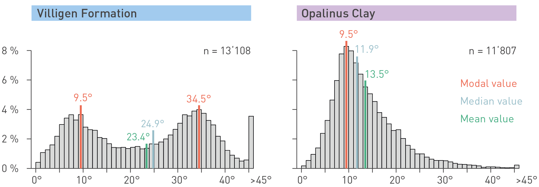
Fig. 6‑33:Histogram and statistical measures of slope gradients within the hillslope domain of JO and surrounding area: two examples

The examples refer to the Villigen Formation (EC 4) and the Opalinus Clay (EC 2) (Ludwig 2018). Slope gradients correspond to pixel-based values from DTM-AV (2-m grid size; © swisstopo). Number ‘n’ indicates the number of pixels for each lithostratigraphic unit. Note that frequencies of values steeper than 45° are summarised in the histograms.

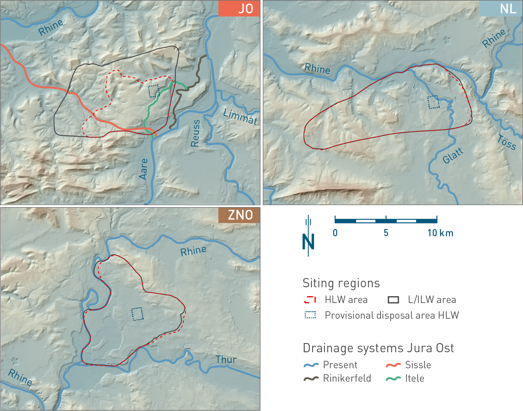
Fig. 6‑34:The siting regions with present-day and alternative main drainage network scenarios

Local topography scenarios based on present-day (all sites) and alternative drainage networks (JO) are considered for the assessment of erosion in the provisional HLW disposal areas at one million years. Potential for lateral changes in drainage scenarios can be drawn from knowledge of fluvial or fluvioglacial processes and denudation.

Lateral migration and changes in main drainage

Lateral migration of the main and tributary rivers, particularly in connection with glacial pro­cesses, can lead to the formation of new drainages by cutting through bedrock relief. These processes are more likely in lower relief landscapes and under the influence of large foreland glaciations (see Fig. 6‑22b in Section 6.4.1.3). However, even in areas of high local topography, corresponding scenarios cannot be excluded over long time periods and are thus considered as alternative evolutions, especially for JO (Fig. 6‑34). Modelled scenarios are the reactivation of the Rinikerfeld Channel, an Aare shortcut using the Sissle drainage with and without incor­poration of the Reuss and Limmat Rivers along this new route, and a breakthrough channel following the Itele Valley. Because the relief (local topography) in the relevant parts of NL and in ZNO is too low to provide meaningful alternative scenarios for modelling of future landscape evolution, a (worst-case) scenario is added that assumes a main drainage developing just above the provisional disposal area. In this case, the remaining overburden thickness is directly derived from the SPIM output of fluvial incision modelling (Section 6.4.3.1).

Modelling results

The first set of results considers a stable main drainage system (Fig. 6‑35, Fig. 6‑36). Such a situation may be expected in an evolution lacking major foreland glaciations. Compared to the results of remaining overburden thickness with respect to the local erosion base (Section 6.4.3.1, Fig. 6‑32), the integration of local topography has a significant positive effect for JO.

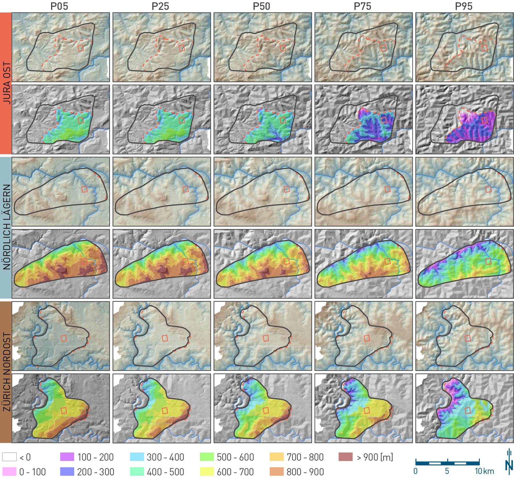
Fig. 6‑35:Results of modelling the evolution of local topography at one million years using the present-day drainage network

Shown are examples of synthetic future landscapes and colour-coded remaining overburden thickness for each siting region and for certain quantiles of parameter combinations (e.g. 25^th percentile of fluvial incision after one million years as derived from the SPIM modelling, combined with the 25^th percentile of the erodibility distributions). Remaining overburden thickness is shown with respect to the Top Opalinus Clay. Red square shows the location of the provisional HLW disposal area.

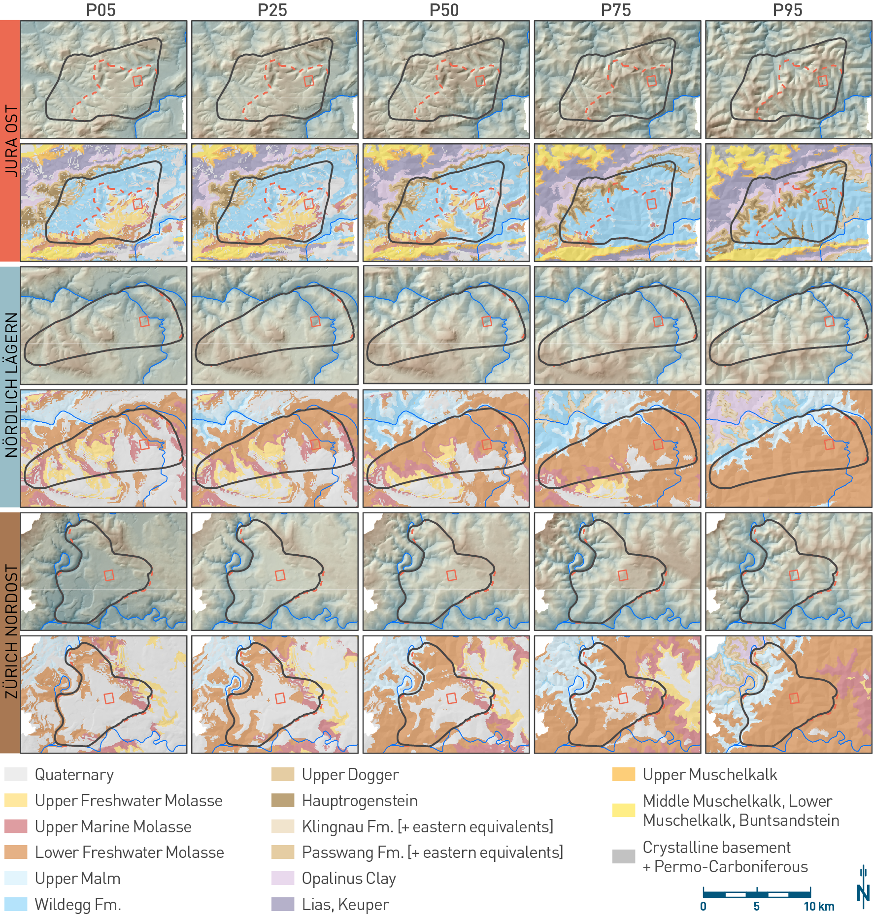
Fig. 6‑36:Outcrop maps representing the evolution of local topography at one million years using the present-day drainage network

Shown are examples of synthetic future landscapes and colour-coded geological outcrop maps for each siting region and for certain quantiles of parameter combinations (e.g. 25^th percen­tile of fluvial incision after one million years as derived from the SPIM modelling, combined with the 25^th percentile of the erodibility distributions). The outcrop map is based on the Regional 3D Geological Model 2012 (Gmünder et al. 2013) used within MuddPILE. Red square shows the location of the provisional HLW disposal area.

In a second step, changes in the main drainage routing in JO (Fig. 6‑34), which might be linked to future foreland glaciations, have been evaluated (Fig. 6‑37 and Fig. 6‑38). When including these alternative drainage networks, it can be seen that the Itele scenario in particular modifies the topography above the provisional disposal area in JO significantly and reduces the remaining overburden thickness considerably (Fig. 6‑37). The probability of occurrence of this scenario, however, is low and depends on the development of a large foreland glaciation (Nagra 2024k).

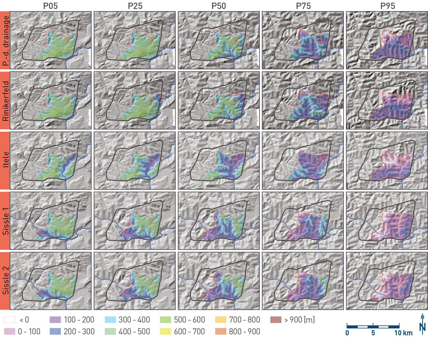
Fig. 6‑37:Results of modelling the evolution of local topography at one million years using alternative drainage networks for JO

Shown are examples of synthetic future landscapes and colour-coded remaining overburden thickness for certain quantiles of parameter combinations (e.g. 25^th percentile of fluvial incision after one million years as derived from the SPIM modelling, combined with the 25^th percentile of the erodibility distributions) for the present-day main drainage network (upper panel) and alternative drainage networks (reactivation of the Rinikerfeld channel, break­through channel through the Itele Valley, a shortcut of the Aare through the Sissle Valley with [Sissle 1] and without [Sissle 2] diversion of Limmat and Reuss). Remaining overburden thickness is shown with respect to the Top Opalinus Clay. Red square shows the location of the provisional HLW disposal area.

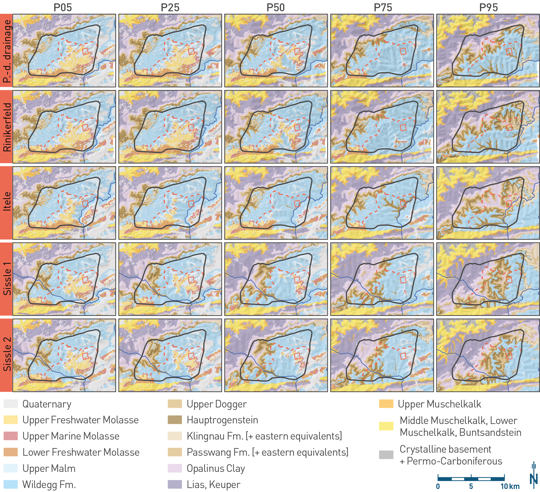
Fig. 6‑38:Outcrop maps representing the evolution of local topography at one million years using alternative drainage networks for JO

Shown are examples of synthetic future landscapes overlain by colour-coded geological outcrop maps for certain quantiles of parameter combinations (e.g. 25^th percentile of fluvial incision after one million years as derived from the SPIM modelling, combined with the 25^th percentile of the erodibility distributions) for the present-day main drainage network and alternative drainage networks (reactivation of the Rinikerfeld Channel, breakthrough channel through the Itele Valley, a shortcut of the Aare through the Sissle Valley with [Sissle 1] and without [Sissle 2] diversion of Limmat and Reuss). The outcrop map is based on the Regional 3D Geological Model 2012 (Gmünder et al. 2013) used within MuddPILE. Red square shows the location of the provisional HLW disposal area.

The actual overburden assessment of the provisional disposal areas with respect to local topo­graphy uses the probability distribution of remaining overburden thickness provided by the surro­gate model (see above, and Nagra 2024k). Results are shown in Fig. 6‑39 for the local topography scenarios in each siting region based on (a) preservation of the present-day drainage network, and (b) including alternative drainage networks. For JO, the latter combines the results for the present-day and alternative drainage networks, as weighted by the expected probability of occurrence (Nagra 2024k). For JO, including local topography in both (a) and (b) has a significant positive effect as compared to accounting for the LEB only (Fig. 6‑32).

For NL and ZNO, alternative drainage networks are assessed based directly on the output of the SPIM model (Section 6.4.3.1), reflecting the probability distribution of the future LEB. For NL, results in (a) and (b), i.e. accounting for local topography vs. for LEB only, are quite similar. The reason is the proximity of the NL provisional disposal area to the present-day main drainage system (defining the LEB), in this case represented by the Glatt River (Fig. 6‑34). Accordingly, less local topography develops at the specific location in the case of a stable main drainage network. In contrast, ZNO shows a higher median value of remaining overburden thickness assuming the present-day drainage compared to NL (Fig. 6‑39a), as its provisional disposal area is more distant to the present-day main rivers. Remaining overburden thickness (including the median), however, is largest in NL among the three sites when including alternative drainages (Fig. 6‑39b). Given the low present-day relief in the eastern part of NL and ZNO, this represents a valid case to compare the two sites with respect to the evolution of local topography. The results are incorporated in the combined assessment of glacial and non-glacial erosion in Section 6.4.4.

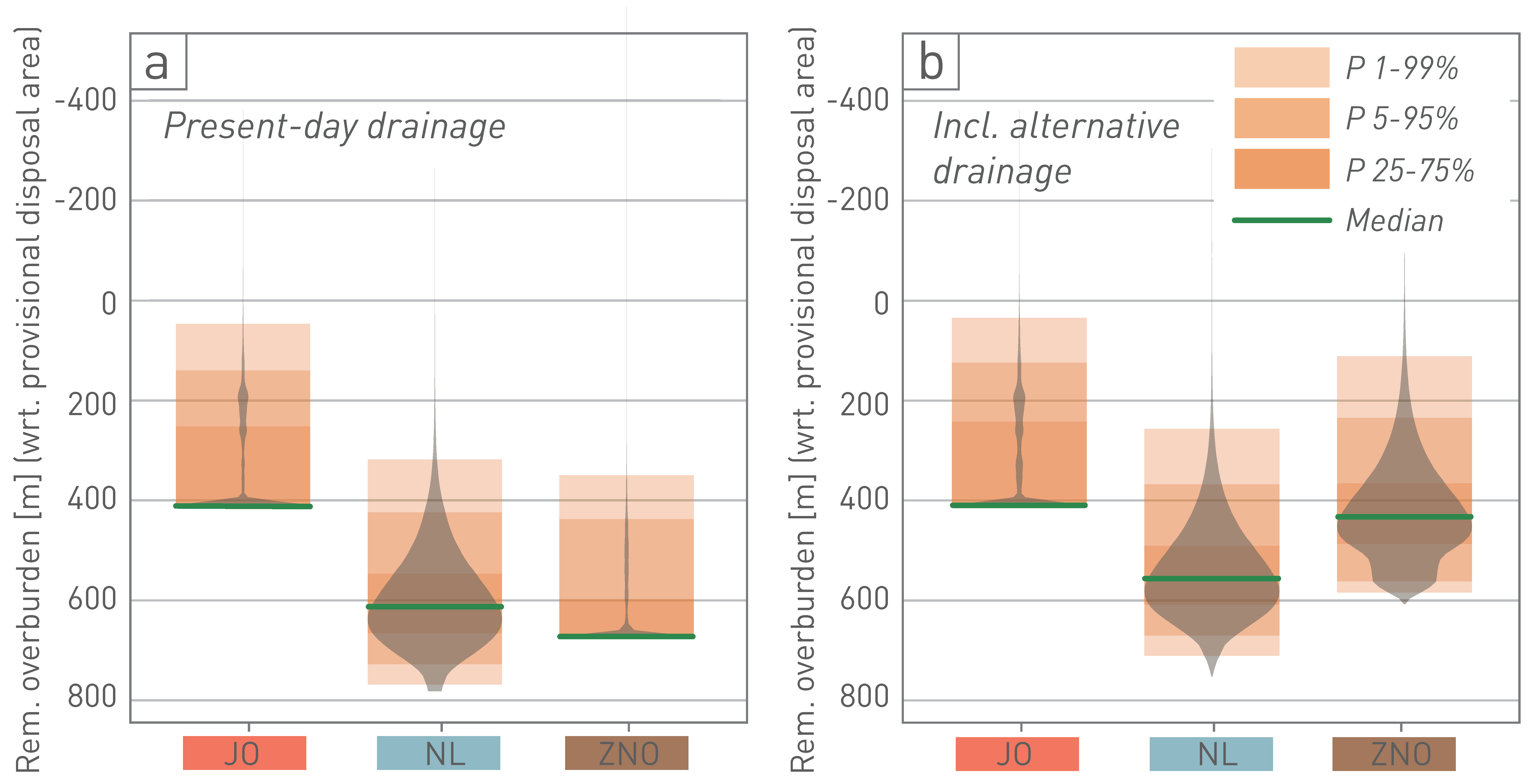
Fig. 6‑39:Distributions of remaining overburden thickness after one million years including local topography for JO

Violin plots and boxes with selected percentiles of remaining overburden thickness at the location of the provisional disposal areas (see caption of Fig. 6‑32 for explanation). (a) Distributions with respect to the evolution of local topography, assuming preservation of the present-day drainage network (i.e. main rivers remain laterally at the same position as today (Fig. 6‑34). Including local topography has a significant effect, especially for JO, if compared to the distribution shown in Fig. 6‑32d. Distributions for JO and ZNO "converge" at the value of the present-day overburden thickness, because of a modelling step that "caps" the model elevation as a function of the present-day terrain surface (further details in Nagra 2024f). (b) Several plausible alternative drainage scenarios were tested for JO (Fig. 6‑34). A respective weighting by the probability of occurrence of the present-day and alternative drainage scenarios is incorporated into the uncertainty estimates for the evolution of local topography in JO. In NL and ZNO, scenarios for alternative drainage networks cannot be reasonably derived because of the low relief. Distributions are calculated using the (worst case) assumption of a main river positioned at the repository location (corresponding to direct out­put from the SPIM modelling, Fig. 6‑32d).

For future deep glacial erosion to affect the geological barrier of a deep geological repository, a series of events must occur. First, a future glaciation has to cover the siting region. Second, the eroded overdeepening must be deep enough to reach the level of the disposal area. This depth is a combination of the future local erosion base, the size and erosion potential of the glaciation, and the incised rock type. Third, the overdeepening must incise at the location of the future repository.

Unlike the simulation of the future local erosion base and local topography, the assessment of deep glacial erosion did not include numerical process modelling. Instead, a chain of calculations using expert knowledge-based parameter distributions link the above outlined aspects of depth, location, and erodibility. These will be summarised in the following paragraphs. For more information see Nagra (2024k).

Key glaciations and future climate

The specific extents of the known principal Quaternary glacials Birrfeld (including LGM), Beringen (probably MIS 6), and Möhlin (probably MIS 12/16) were used as key glacial stages in the future assessment of erosion with respect to the three siting regions (Fig. 6‑18d, Fig. 6‑24, Sections 6.3.1 and 6.4.1.4). The comparison of their respective ice extents with the locations of the siting regions suggests that JO will only be covered by a future glaciation of Möhlin-size, whereas NL would be affected by Möhlin- and Beringen-size glaciers, and ZNO would be affected by glaciers that would correspond to the size of all three principal glaciations. For a full assessment it is also considered that a foreland glaciation might occur, but it is smaller than LGM, i.e. in this context smaller than reaching ZNO. Such a glaciation will not have any impact on the estimated deep glacial erosion. The concept of key glacials was used to (1) estimate the probability of occurrence of alternative drainage scenarios (see Section 6.4.3.2) conditional on the occurrence of a key glacial; (2) to estimate the overdeepening depth for each of the key glacials; and (3) to estimate the probability of occurrence of future glaciations with similar extents as the key glacials over a time span of one million years. The Quaternary glaciation history of Northern Switzerland and the model results estimating ice volume in the next one million years (Talento & Ganopolski 2021; see Fig. 6‑17 in Section 6.3.3.1) served as guidance for the latter argumentation.

According to Figure 19 in Preusser et al. 2011, there may have been four larger ice advances of "key glacial" size (1× Möhlin-size, 1× Beringen-size, 2× LGM-size [Habsburg and LGM]), see also Section 3.5. Earlier glaciations did reach the foreland, as rarely indicated by intercalated till within Deckenschotter deposits. It seems, however, that the above-mentioned four larger glaciations took place only after the accumulation of the TDS and probably after (or associated with) the Mid-Pleistocene Transition (MPT), when glacial cyclicity switched from a dominant 41-kyr to a 100-kyr cycle (Section 6.3.1). The ages of the Möhlin and Beringen Glacials are not unambiguously resolved, but the Möhlin Glacial is tentatively assigned to MIS 16 or MIS 12 and the Beringen Glacial to MIS 6 (see Section 3.5). Because of the age uncertainty and general poor preservation of continuous geomorphic markers for the Möhlin ice extent, it cannot be excluded that the ice advanced far to this position during both, MIS 16 and MIS 12 times. Many of the overdeepened throughs observed in the external Swiss Alpine Foreland are thought to be associated with these abovementioned large glaciations (Section 6.4.1.4). In summary, this suggests that the overdeepenings observed in Northern Switzerland are the cumulative result of recurrent processes that have affected Northern Switzerland during the past ~ 800 kyr or more, which corresponds roughly to the time frame to be assessed for the future. Accordingly, the observed overdeepening depth could be considered an "implicit stack", i.e. overdeepening depth at one million years may similarly reflect the cumulative result of multiple foreland glaciations. Because the depth distribution is placed below the future local erosion base, the most influential overdeepening with respect to its potential to erode down to the repository level, is one that occurs late (when the local erosion base is already lowered significantly), and which stems from a large glaciation with high glacial erosion potential (see Nagra 2024k for more details).

Because of continuous erosional downcutting and subsequent decrease of the accumulation area of future glaciers, future foreland glaciations may be smaller even with similar climate forcing (Egholm 2022).

Overdeepening depth and dependence on rock type

The glacially eroded Molasse assemblage in Northern Switzerland comprises a variety of differ­ent, yet mostly easily erodible rock types. Because most of the observed glacial overdeepenings were carved into Molasse rocks (Section 6.4.1.4), these strata were considered as the base unit, when evaluating the potential depth of future overdeepenings. For each key glacial to be consid­ered per site, a reference (i.e. for Molasse rocks) depth distribution for future glacial overdeep­ening occurring within each HLW perimeter, respectively was established during SHELF-based workshops (Fig. 6‑40; see Nagra 2024k for detailed distributions and discussion).

The main evidence used to estimate the uncertainty of future glacial overdeepenings is based on the statistics of observations in Northern Switzerland, supported by global observations (Nagra 2024k). In this context, it is important to note that for instance the overdeepening depth drilled in the Nagra boreholes is contained within the total assumed probability but may correspond to a less likely percentile (Fig. 6‑40; e.g. QHST in NL would be near the 70% percentile of the assessed probabilities for a future Beringen or Möhlin key glacial). These boreholes were explicitly located to drill the deepest parts, while the majority of the glacial overdeepenings in the distal foreland is shallower (e.g. Section 6.4.1.4, Fig. 6‑24, Fig. 6‑25, Fig. 6‑26, Fig. 6‑28, see Nagra 2024k for more statistics). The width of the total assumed probabilities allows no over­deepening at all on the lower bound and a depth similar to the exceptionally deep Bodensee Trough on the upper bound (Fig. 6‑40). Such large depths, however, are considered very unlikely.

The assumed total probabilities of reference overdeepening depth for Möhlin and Beringen key glacials in NL and ZNO closely resemble each other but for a slight shift towards larger depth for future Möhlin-size glacials. The argumentation here is based on the remaining age uncertainty with respect to the sediment fill of the overdeepenings and thus the preceding glacial erosion event. In addition, the close proximity of similarly sized troughs, which may reflect different glacials (e.g. Strassberg Through [presumably Möhlin erosion] next to the Bülach Trough [presumably Beringen erosion] in the lower Glatt Valley or Marthalen Through [presumably Möhlin erosion] next to the Andelfingen Trough [presumably Beringen erosion] in the lower Thur Valley; Fig. 6‑26b and c; Buechi et al. 2024) does not allow a clear distinction between the erosional efficiency of Beringen and Möhlin Glacials. The limited bedrock incision of an LGM-size glacial is also reflected in the total assumed probabilities but allowing also deeper values with less likely occurrence, because of the observation of glacial erosion during the similarly sized Habsburg Glacial in the Birrfeld Trough (Section 6.4.1.4).

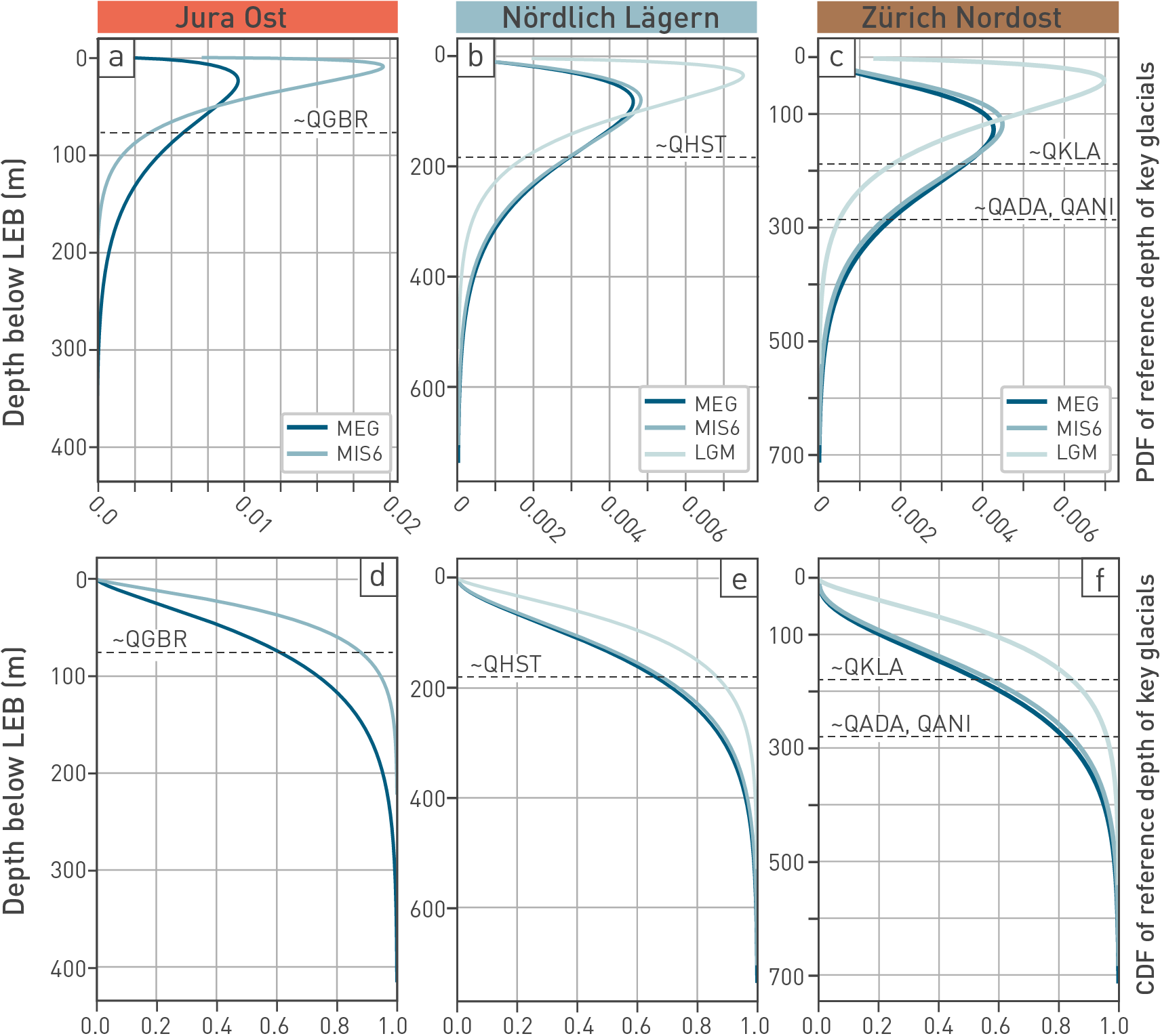
Fig. 6‑40:Total assumed probabilities for reference overdeepening depth per key-size glacia­tion

Total assumed probabilities for reference depth distributions (Molasse) for each site and the respective key glacial. Note that MIS 6 refers to the Beringen glaciation and MEG to Möhlin. Figures in the upper panel show the probability density function (PDF), those in the lower panel show the respective cumulative distribution function (CDF) for Jura Ost (left), Nördlich Lägern (centre), and Zürich Nordost (right). Horizontal dashed lines correspond to the approximate depths (below LEB) of Quaternary boreholes that Nagra drilled within the wider areas of the siting regions (Section 6.4.1.4). QGBR: Gebenstorf-Brüel borehole is located within the lower Aare Valley but not within the HLW area of JO. QHST: Hochfelden-Strassberg borehole is located in the southernmost part of NL. QKLA: Kleinandelfingen-Laubhau borehole is located in the southernmost part of the ZNO-HLW area. QADA: Adlikon-Dätwil borehole is located in the south, just outside of the ZNO-HLW area. QANI: Andelfingen-Niederfeld borehole is also located in the south, just outside of the ZNO-HLW area (for references, see Tab. 2‑2).

Because observations show that overdeepenings tend to incise into easily erodible rocks, if they are not additionally restricted by topography (see Section 6.4.1.4), and are less deep within more resistant rocks in such cases, a scaling was introduced leading to a stretching or shortening of the reference depth distribution if incision reaches a different rock type. Accordingly, the erodibility classes were scaled with respect to the Molasse assemblage (Fig. 6‑41). For example, rock types that are part of EC 4 (e.g. Malm limestones) were considered on average only half as erodible as Molasse-type rocks.

Nevertheless, even if less likely, certain conditions might occur where resistance to erosion per class differs from the bulk of the material. The consideration of such possibilities is visible in the overlaps between the probability density functions (PDF; Fig. 6‑41a, see Nagra 2024k for more detail).

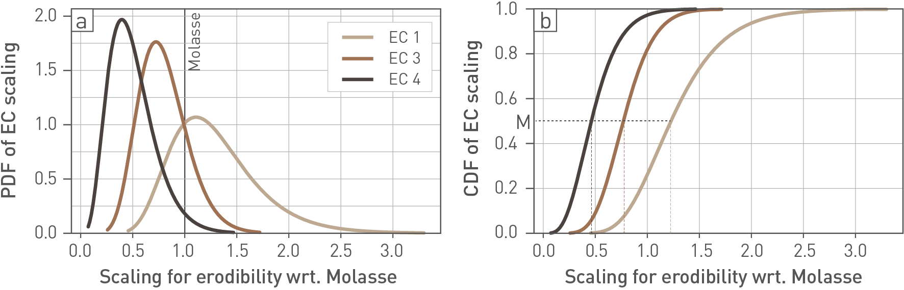
Fig. 6‑41:Total assumed probabilities of erodibility scaling with respect to the Molasse of Northern Switzerland

The sediments of the Molasse assemblage of Northern Switzerland with their variety were considered as the base unit with the scaling value of 1.0 (labelled in a). Molasse sediments are in erodibility class (EC 2). Accordingly, rock types in EC 1 are generally easier to erode, and rocks in EC 3 and EC 4 are harder to erode. Probability (a) and cumulative distribution function (b) are based on expert judgement under the prerequisite that the median values (M, labelled in b) follow the assumption of M(EC 1) > M(EC 2 [equals Molasse]) > M(EC 3) > M(EC 4).

By taking the rock types at a certain overdeepened point into account and by scaling the reference depth of incision based on these rock types, the distribution for the actual depth of overdeepening at that point can be evaluated. Note that this distribution is conditional on glacial overdeepening occurring at the selected point (and conditional on a specific LEB). For evaluating the unconditional probability of repository excavation due to glaciation, additionally, the probability of future glaciation events, the spatial occurrence of glacial overdeepening and the actual over­deepened area must be taken into account (see next subsection). The full stepwise procedure to evaluate probabilities of incision (fluvial and deep glacial) at a certain point is illustrated in Fig. 6‑42.

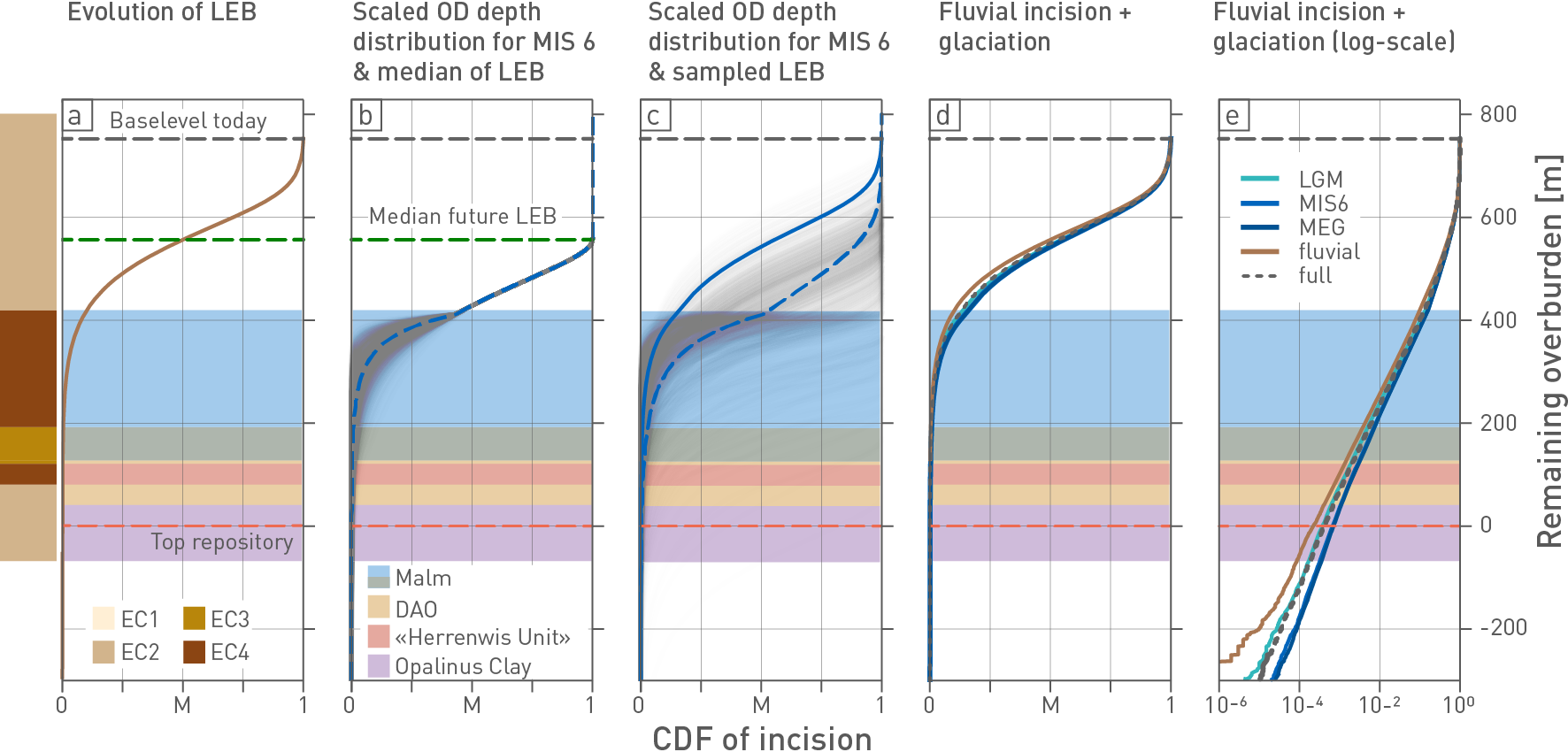
Fig. 6‑42:Step-wise illustration of procedure to evaluate the probabilities of fluvial and deep glacial erosion at a certain point

The illustration represents a step-wise visualisation of the probabilistic approach for the example of NL and the timing of one million year. The stratigraphic column below the Molasse is shown in all subfigures. The (colour-coded) associated erodibility classes are visible on the left. (a) Cumulative distribution function (CDF) of the future local erosion base (LEB, dashed green line shows median value). (b) Scaled depth distribution (CDF), exemplarily shown for a future MIS 6 (Beringen-size) glaciation linked to the median of the future LEB (dashed green line), derived by scaling the reference depth distribution (dashed blue CDF) with different sets of scaling factors sampled from their distributions (Fig. 6‑41). The variability resulting from the scaling starts at the depth of the stratigraphic step between Molasse rocks and rocks of EC4 (grey lines). Note that this is a subset of the full samples and plotted only for illustration purposes. (c) Scaled depth distributions (grey CDF) for different samples of the future LEB (blue solid CDF). The blue dashed line corresponds to the resulting CDF conditional on the glaciation and the occurrence of an overdeepening (OD) scenario at the location of the provisional disposal area. It does not involve the condition of an actual OD at the location¹⁸. This distribution is calculated conditional on the occurrence of a glacia­tion comparable to the one during MIS 6. (d) Probability of incision (fluvial and glacial) for a certain remaining overburden thickness, including all key glacials with their probabilities of causing overdeepening within the provisional disposal area. The process termed fluvial erosion (‘fluvial’) describes the case of no glacial OD, e.g. for glaciations of a size smaller than during the LGM and corresponds to the distribution of the future LEB. (e) For better visibility, the incision probability (same as in d) is illustrated in log-scale. Note that in this illustration it is assumed that glacial overdeepening occurs directly above the provisional disposal area.

Locations of future glacial overdeepenings

Besides the occurrence of a glaciation with a certain (key-size) extent and the depth of a future overdeepening, the potential location of future overdeepenings must be assessed. This is done by combining and weighting different scenarios.

The multiphase infilling history of many deep glacial troughs suggests a tendency for reoccupa­tion of existing overdeepenings. Present overdeepenings as potentially preconditioned pathways for future reoccupation are thus one scenario. A spatial buffer around the present-day over­deepenings to account for growth in length or width and allowing a lateral shift of the axis, and thus the location of deepest erosion, can be applied. However, the potential for glacially diverted channels with new overdeepenings cannot be excluded as a scenario and this is thus integrated within the probabilistic model. Although the future topography cannot be precisely forecasted, there are certain assumptions that help in deriving such potentially additional scenarios. Topo­graphic steering of ice through pre-existing valleys (ice is probably steered away from hills and ridges into already existing troughs and valleys; Kessler et al. 2008) is considered in the scenario building. On the contrary, the lower the relief, the more degrees of freedom or randomness need to be accounted for. This is especially important for ZNO but also the eastern part of NL, where the present relief is low. A set of plausible scenarios for each site was ranked during SHELF-based workshops, which in turn provided the input for scenario maps (Fig. 6‑43, see Nagra 2024k for more details). The darker the colour in these maps appears, the more likely a certain scenario becomes. Calculations of remaining overburden thickness that incorporate the influence of over­deepening locations are shown in Section 6.4.4.

Finally, it is important to note that while the coloured parts of the maps highlight where over­deepening might plausibly occur, the actual dimension of the overdeepenings within such a zone is significantly smaller (compare the present-day occurrences in Fig. 6‑24). For instance, ~ 5% of the NL siting region and less than 18% in ZNO are actually overdeepened. Because of a narrowing of the overdeepening forms towards depth, this number decreases, if considering only deeper troughs. For instance, overdeepenings of more than 50 m below LEB constitute ~ 2% area in NL and ~ 6% area in ZNO (see Nagra 2024k for more details). Such fraction of actual over­deepening with a potential overdeepening scenario is considered in the model (see Nagra 2024k) and results in an additional reduction of overdeepening probability.

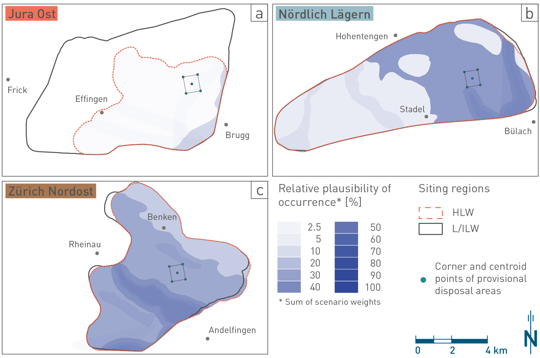
Fig. 6‑43:Scenarios for spatial occurrence of future overdeepenings within the siting regions, one million years

Shown are colour-coded maps with darker colours reflecting a higher plausibility of occur­rence of future glacial overdeepenings in the JO (a), NL (b) and ZNO (c) siting regions. The provisional disposal areas are shown with their respective corner and centroid points. For JO, overdeepening to occur is less likely for the next one million years. Here, the generally less likely occurrence of overdeepening is strongly linked to the (alternative) drainage scenarios (see Section 6.4.3.2).

This section presents the combined results of the erosion assessment for a 1-million-year time frame. Discussed are the remaining overburden thickness for the expected geological evolution as well as the probability of combined glacial and non-glacial repository excavation. The example below considers the full range of uncertainties as elicited for the locations and depth of the provisional HLW disposal areas over the period of one million years. Of this full range of uncertainties, the 5 – 95% range is considered as "expected range" of future evolutions. In Nagra (2024k), additional calculations are shown for subsets of scenarios that feed into site comparison (site comparison criteria 2.2. and 3.3; Nagra 2024t).

Fig. 6‑44 shows the total probabilities of remaining overburden thickness distributions after one million years. Remaining overburden thickness is calculated in a Monte-Carlo approach using one million samples (Section 6.4.2.3, Fig. 6‑29) and is provided with respect to the respective provisional disposal areas (i.e. the worst case of their four corner- and one midpoint¹⁹ ). The respective probabilities to incise to the depth of the provisional disposal areas are deduced from the Monte Carlo samples. Fig. 6‑44 is tripartite for better accessibility: the upper panel provides probability density functions (PDF), from which the most likely scenarios can be deduced (bulk of the curves, highlighted by the vertical arrows). The middle panel shows the same distribu­tions as cumulative distribution function (CDF). The shaded areas represent the 5 – 95% pro­bability (x-axis) and associated overburden thickness amounts (y-axis), which are considered here as "expected range" of future evolutions. Very low probabilities are not distinguished in the upper and middle panels. Therefore, the lower panel shows the CDF in log-space. The intercept with the position of the provisional disposal area (red dashed line) reveals the probability of excavation.

The most likely scenarios show at least ~ 400 m of remaining overburden thickness above the repository after one million years at all sites (vertical arrows in Fig. 6‑44a). In NL, nearly 600 m of overburden thickness is likely to be preserved. At the 5 – 95% probability range, between ~ 125 and 410 m of overburden thickness might be expected in JO, between ~ 350 and 670 m in NL and between ~ 220 and 560 m in ZNO (shaded area and vertical arrows in Fig. 6‑44b). Considering the required 200 m of overburden thickness for efficient self-sealing (Section 5.7), the JO site (i.e. at the position of the provisional disposal area) shows more limitations within this range than the other sites. However, suitable conditions in JO are available in the immediate surroundings of this provisional disposal area (Nagra 2024k), such that JO can also reliably provide sufficient overburden thickness to secure the barrier function over the period under consideration.

Excavation of the repository within one million years was estimated to be highly unlikely at the provisional disposal areas in all three siting regions. This fact is best seen in the log-scale visualisation of the distribution (vertical arrows in Fig. 6‑44c, see grey box showing the 5 – 95% range for comparison). This likelihood is about an order of magnitude lower for the provisional disposal area in NL than in JO and ZNO. Excavation probabilities were calculated to show the robustness of the repository. A discussion on the plausi­bility of the corresponding results, especially considering the extreme values contained in the tails of the total probability can be found in Nagra (2024k).

Fig. 6‑44 also shows the main contributor with respect to the distributions of remaining over­burden thickness. Although deep glacial erosion is capable of incising strongly into the over­burden, its probability to incise at the position of the repository is strongly reduced. The main contributors consequently are fluvial incision driven by rock uplift and, in case of JO, associated evolution of local topography. The present-day low relief in ZNO and in the east of NL does not allow to reasonably consider and rank scenarios for future evolution of local topography. Instead, remaining overburden is considered with respect to the local erosion base (see Section 6.4.3.2). However, it cannot be excluded that the location of the main drainage will be shifted away from the provisional disposal area and a significant protective relief will develop in the future. Accordingly, the remaining overburden thickness might be further increased, and the probability of excavation further reduced in NL and ZNO.

Consequently, considering the three erosion processes, NL provides the best protection against future erosion.

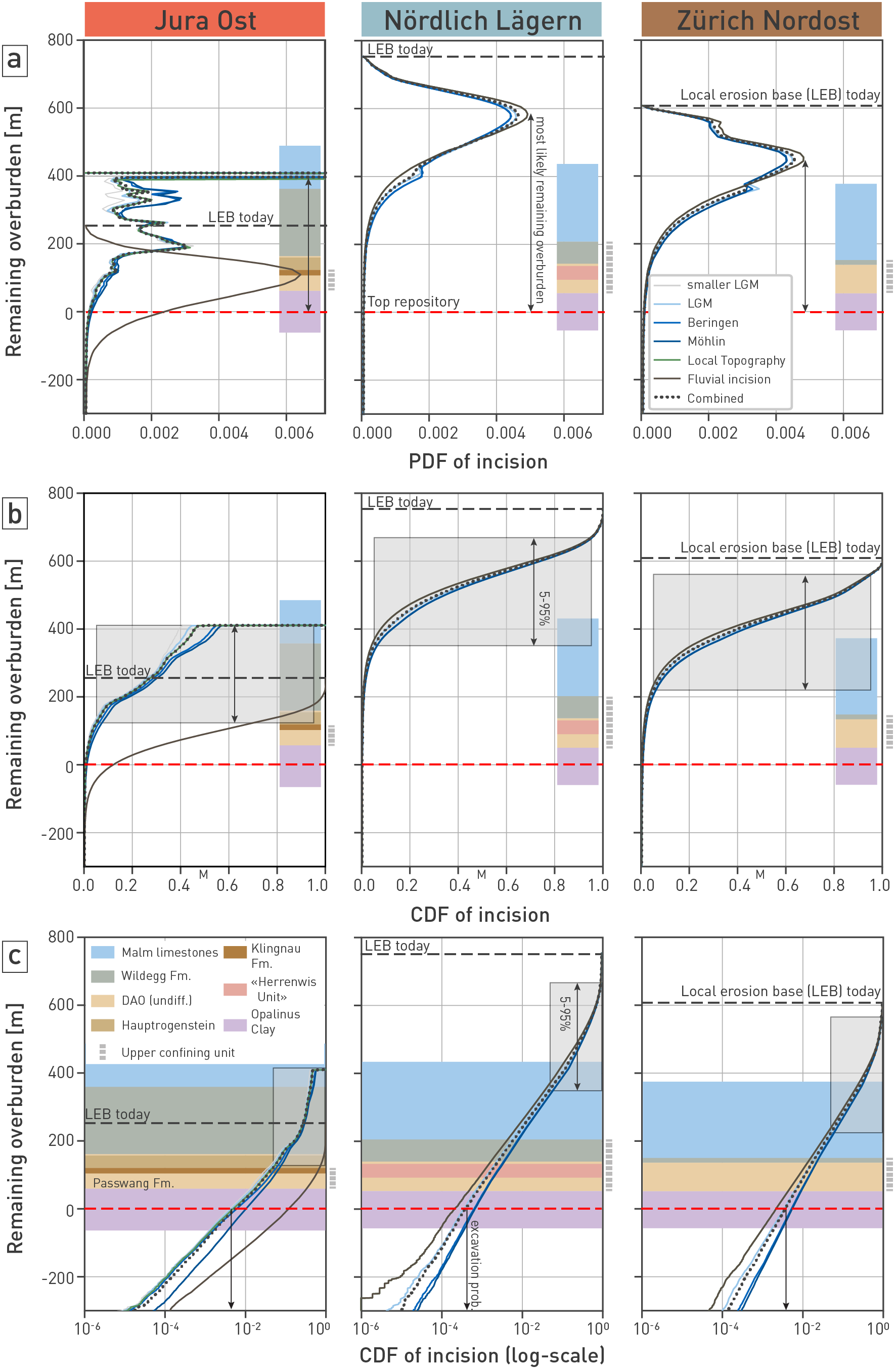
Fig. 6‑44:Estimated probabilities of remaining overburden thickness above the provisional disposal area in the three siting regions

The same outputs are displayed in three different formats for better visualisation (a) as probability density function (PDF), (b) as cumulative distribution function (CDF), and (c) as CDF, transferred onto a logarithmic scale. Results are shown with respect to the depth and location of the provisional disposal area (red dashed line). The thick black dotted line represents the final combined probability. That is, it integrates over (i) both glacial and non-glacial pro­cesses and (ii) the occurrence of all considered key glacials. The lines "smaller LGM", "LGM", "Beringen" and "Möhlin" integrate over both glacial and non-glacial pro­cesses but are restricted to the occurrence of the specific key glacial. The line "Local Topo­graphy" integrates over all considered key glacials for determination of alternative drainage networks but is restricted to non-glacial processes (output Model B, i.e. no glacial over­deepening). The line "Fluvial incision" describes the modelled LEB (local erosion base) from Model A.

For JO, the final combined curve is a combination of the fluvial incision by main rivers (line "Fluvial incision"), evolution of local topography (including ranked scenarios) and deep glacial erosion (output Model C; conditional on the occurrence of key glacials). Local topography was not included in the case of NL and ZNO. Here, a main river (defining the local erosion base) was assumed to be located directly above the provisional disposal area (see Section 6.4.3.2). The vertical arrows in (a) highlight the most likely amount of remaining overburden thickness at the location of the provisional disposal area, in (b) the 5 – 95% range (also shaded), see M for position of median values, and in (c) the probability of excavation, which is about an order of magnitude lower in NL (see grey shaded box showing the 5 – 95% range for comparison). Simplified lithostratigraphic columns are provided with these images, allowing to visualise the incision depth. DAO: Dogger Group above Opalinus Clay. The grey dotted bar at the right of each subfigures represents the upper confining units.

Considering the erosion assessment aimed at ensuring uncompromised barrier properties during the period under consideration, the following conclusions are drawn:

• The overall knowledge about the capability, timescales, form and rate of erosion processes, and the erosion history of Northern Switzerland have been improved considerably by detailed field and laboratory work during recent years. The effects of recurring climate-driven erosion processes superposed on the low-strain domain of Northern Switzerland have been identified and analysed with respect to landscape evolution. Nevertheless, age determination and the limited availability of dated Quaternary geomorphic markers and sediments (e.g. Decken­schotter, infills of glacially overdeepened valleys) remain a challenge. Consequently, the age uncertainties of Quaternary landforms and deposits are accounted for in a systematic assessment of future erosion.

• Future erosion processes (glacial and non-glacial) are expected to be generally comparable to processes that have repeatedly influenced the area of the siting regions during the Quaternary, but they are inferred to operate at lower rates. One main argument for slower future process rates is the formation of smaller glaciers and a delay in glacial inception because of anthropogenic CO₂ emissions. In addition, analyses of the fluvial topography show that the catchment of the Rhine River will grow at the expense of the Danube catchment, thus no major pulse of drainage reorganisation will cause deep incision as the major wave of retrogressive erosion of the Rhine has already passed by the area of the three siting regions. In addition, less erodible rocks in the stratigraphic sequence below the Molasse strata are predicted to slow down erosion further.

• The assessment of future erosion was done using a robust, structured hybrid-probabilistic approach, based on available field data, rate determinations, laboratory tests and modelling, to evaluate the behaviour of the erosional system in Northern Switzerland for different future scenarios.

• A residual cover thickness of 200 m as required for maintaining the self-sealing properties of the Opalinus Clay can be shown for the most likely scenarios in all the siting regions for the period under consideration. Using the 5 – 95% range as reference, the JO site shows more limitations for such a 200 m criterion at the location of the provisional disposal area. How­ever, suitable conditions in JO are available in the immediate surroundings of this provisional disposal area, such that JO can also reliably provide sufficient overburden thickness to secure the barrier function over the period under consideration. Nevertheless, because of the com­parably small distance between the repository depth and the local erosion base, JO is dependent on the preservation of the local topography and is thus more sensitive to changes in the fluvial network compared to the other sites. The NL site is a well-suited location for the development of a repository because it is protected against future erosion from all of the principal erosion processes capable of causing deep incision by the large emplacement depth.

• Fluvial incision, driven mainly by rock uplift, dominates the modelled overburden thickness assessment on a timescale of one million years. Although deep glacial erosion can greatly increase the degree of incision, it is less likely at the sites. This is because of the low pro­bability of glacial overdeepenings occurring at the location of the provisional disposal area, the more resistant rocks below the Molasse strata, and the longevity of elevated atmospheric CO₂ concentrations that are predicted to delay future foreland glaciations. Because of conti­nuous erosional downcutting and subsequent decrease of the accumulation area of future glaciers, foreland glaciations might be smaller even with similar climate forcing.

• Excavation of the repository by erosion within the next one million years can be considered extremely unlikely in all the provisional disposal areas but is nearly an order of magnitude lower in NL.

Future geodynamic evolution (Section 6.2), changing climate (Section 6.3) and morphological changes due to erosion (Section 6.4) can alter hydrogeological and hydrogeochemical conditions (states, properties) and might ultimately affect barrier efficiency. Consequently, the evolution of the barrier system over the period under consideration needs to be addressed. This section dis­cusses the most relevant hydrogeological and hydrogeochemical changes in the aquifer-aquitard system:

• Changes in flow systems in the deep aquifers (Malm, Hauptrogenstein, Keuper and Muschel­kalk aquifers; Section 6.5.1)

• Changes in hydraulic barrier efficiency of the host rock and low-permeability confining units (Section 6.5.2)

• Changes in diffusion properties (Section 6.5.3)

• Changes in porewater composition and related effects on solute mobility (Section 6.5.4)

• Changes related to dissolution processes below the host rock (Section 6.5.5)

• Alteration of host rock mineralogy (Section 6.5.6)

Note that the evolution of the biosphere, including scenarios and parameters for the evolution of shallow aquifers and surface waters, is discussed in a separate report (Nagra 2024q).

The host rock and confining units are sandwiched between aquifers that provide the hydraulic and hydrogeochemical boundary conditions to the low-permeability sequence (Section 4.5.3.1, Fig. 4‑84). Malm and Hauptrogenstein constitute the relevant aquifers above the host rock. Below the host rock, the local Keuper and the regional Muschelkalk aquifer are relevant. During the period under consideration, the flow systems in these deep aquifers can be affected by a variety of processes. In the following subsections, the impact of the most important drivers is briefly discussed.

Groundwater recharge is dependent on climatic conditions, in particular temperature and precipi­tation. Changes in these parameters strongly impact water flux and residence time in shallow aquifers. In comparison, the impact on deep flow systems is dampened because of the lower hydraulic conductivities and because the overall differences in hydraulic head driving these deep systems are not strongly affected by recharge. Climate-related changes in recharge conditions thus have a subordinate influence on deep flow systems compared to other processes of the long-term geological evolution. Note that the impact of glaciations and perma­frost is discussed separately (Section 6.5.1.3).

Over timescales of 10⁵ to 10⁶ years, erosion may significantly modify the morphology of Northern Switzerland (Section 6.4). There will be a general lowering of the river network with respect to the repository depth (Fig. 6‑32) and a decrease in the overburden thickness above the different aquifers (Fig. 6‑35 to Fig. 6‑38). The hydrogeological system will tend towards increasing flow rates in the aquifers as well as decreasing groundwater salinity and groundwater residence times over a timescale of 10⁶ years because of the increasingly shallower situation and related decom­paction effects. Ultimately, when the carbonate rocks have been uplifted above the baselevel (Fig. 6‑32; e.g. Hauptrogenstein in JO), they may be affected by epigenic karst development.

Over the period under consideration, erosion will drive the development of more active flow systems and a shortening of discharge path lengths for the Malm aquifer in the NL and ZNO siting regions. This effect will probably be smaller or occur later in NL because of the greater depth of the Malm aquifer (see also Section 4.5.6).

In the JO siting region, the aquifer above the host rock (Hauptrogenstein) may be affected by decompaction effects and by potential dissolution as river incision may position the aquifer above the local baselevel (Fig. 6‑32, Fig. 6‑38). The less likely drainage evolution scenario assuming a direct connection of the Aare Valley to the Sissle for instance (Section 6.4.3.2) may result in an important reorganisation of the local hydrogeological system, with the new valley acting as a major discharge area for the Hauptrogenstein aquifer.

For the aquifers below the host rock, the remaining substantial overburden thickness will result in negligible changes in the aquifer properties within the siting regions (see also Section 6.4.4).

During cold climate periods, the hydrogeological conditions may be affected by glaciation and permafrost (Section 6.3).

Water pressure below glaciers (warm-based, Section 6.3.2) increases with increasing ice thick­ness. A synthesis of studies in North America and Europe suggests that subglacial recharge may be increased by as much as 2 – 6 times compared to modern levels (Person et al. 2012). Such recharge may induce substantial changes in terms of water fluxes, hydraulic gradients, residence times and flow directions, as well as isotopic composition of the groundwaters. The depth to which this water infiltrates depends on numerous factors, such as the thickness of the ice, the duration of the glaciation and the hydraulic properties of the units below the glacier.

There is evidence from the study area of the effects of past glaciations on the hydrogeological system. In the Bodensee area, which was covered by substantial ice thicknesses in the past (Section 6.3.2), the groundwaters from the Malm and Molasse aquifers show a distinct cold climate isotopic signature, probably caused by increased subglacial recharge during the last glaciation period (Section 4.5.5.2, Fig. 6‑45). Note that today this area is considered to be a discharge area. In the Swiss Molasse Basin further to the south, water types change with increasing depth and include Molasse groundwaters that infiltrated during Pleistocene cold time periods (Waber & Traber 2022). In the siting regions, no evidence exists for such glaciation-induced cross-formation recharge processes into the Malm aquifer (Section 4.5.5.2). This may be because of lower ice thickness and shorter duration of glaciation (Fig. 6‑15), thick coverage by the Molasse sediments or differences in hydraulic conductivities of the Molasse and the Malm aquifer. Numerical simulations for a comparable geological setting in the Bavarian Molasse Basin show that a lower permeability aquifer below the Molasse cover may significantly reduce the depth of subglacial recharge (Schintgen & Moeck 2021). The fact that Malm permeabilities defined in these simulations compare well with the hydraulic conductivities measured in the siting regions of Northern Switzerland (Fig. 4‑88) indicates that the low permeability of the Malm aqui­fer minimises glaciation-induced cross-formation flow across the Molasse deposits into the Malm.

However, a reduction in overburden thickness and subsequent decompaction effects may lead to increased hydraulic conductivities in the Malm aquifer (Section 6.5.1.2), allowing for higher water fluxes and reduced residence times during future glaciations, in particular in the western part of ZNO. In JO, future glaciations are less likely (e.g. Sections 6.4.2.1 and 6.4.3) but could nevertheless affect the Hauptrogenstein aquifer.

In the past, Northern Switzerland was repeatedly affected by permafrost (Section 6.3). Permafrost may reduce or locally prevent recharge and/or discharge through freezing of pathways (e.g. Jost et al. 2007, McIntosh et al. 2012) and thus affect the flow systems mainly in terms of reducing water fluxes and increasing residence times. During the period under consideration, such changes are temporarily expected in all the siting regions.

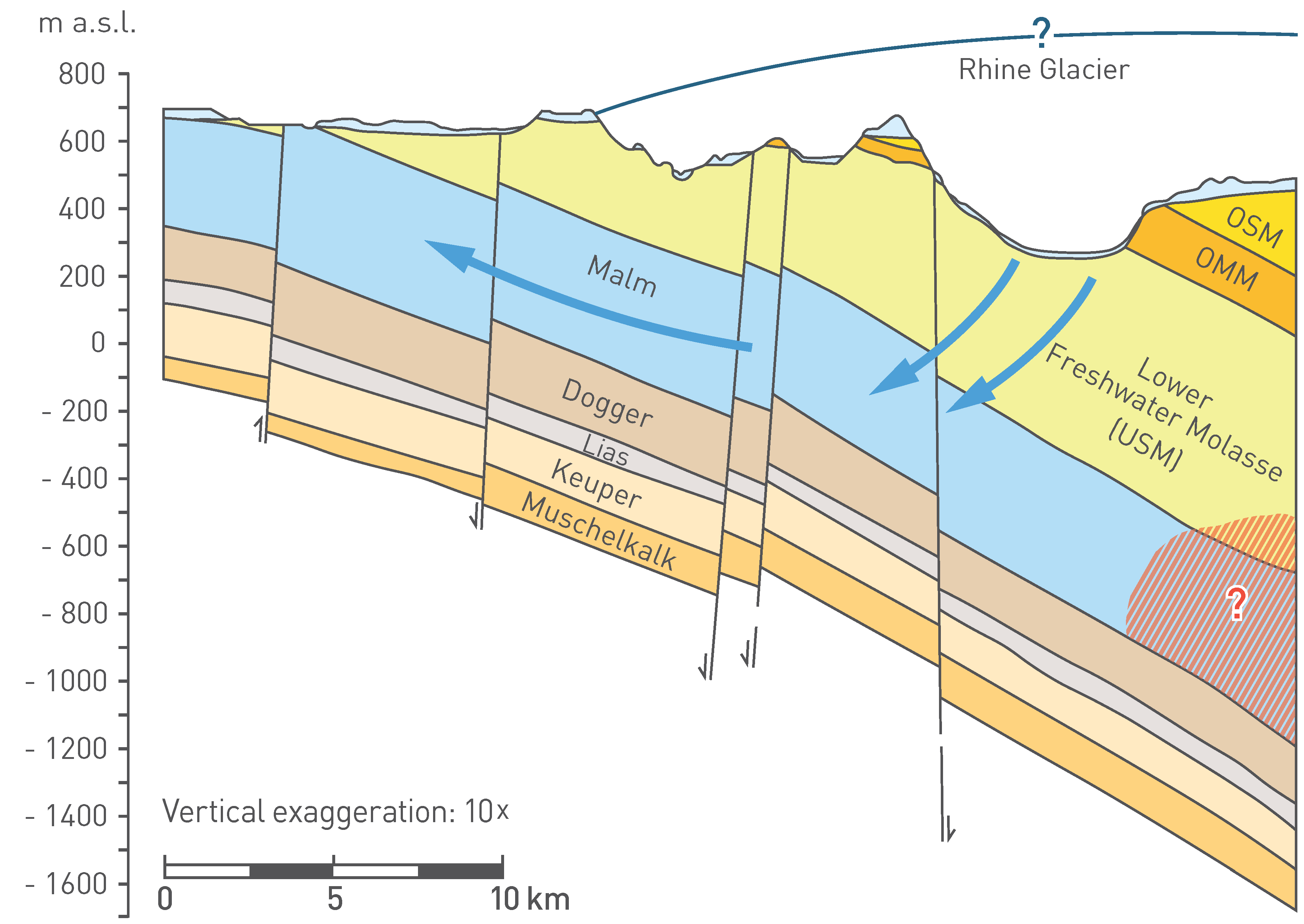
Fig. 6‑45:Schematic representation showing Pleistocene subglacial meltwater recharge into the Malm aquifer in the Bodensee area

Figure from Waber & Traber (2022), based on earlier work of Bertleff & Watzel (2002). Blue arrows indicated recharge of subglacial meltwater into the Malm aquifer. Red hatched area indicates remnants of saline deep groundwaters. Note that there is no indication for such Pleistocene cross-formation meltwater flow across the Molasse in the siting regions. However, cross-formation flow across the Molasse and Malm could become more relevant in the future after reduction of the Malm overburden thickness (see text for discussion).

Strong earthquakes, even with distant epicentres, can induce changes in the groundwater system as evidenced by changed discharge rates of groundwater springs or fluctuations in groundwater levels in boreholes (Nagra 2024i, Wang & Manga 2010). Such changes may be the result of stress changes and related dilation, or contraction of cracks or enhanced permeability produced by seismically induced fractures. The effect generally diminishes over the timescale of a few years. It is thus not expected that effects of single earthquakes would fundamentally and persistently change the flow system.

Accumulated slip along faults can also affect aquifer pathways. Fundamental persisting changes to the aquifer flow system due to fault slip on regional or local faults are not anticipated during the period under consideration as deformation rates are generally low (Section 6.2). Nevertheless, the impact of flow across and along faults on the deep aquifer system and on discharge paths and the effects on flow paths and discharge areas are discussed in Nagra (2024n).

The magnitude of the vertical hydraulic gradient across the host rock and the entire aquitard sequence influences the advective water flux. In this section, two bounding cases are discussed: In the first one, the hydraulic gradient is controlled by the difference in hydraulic head between the aquifers above and below the low-permeability sequence. This case would be relevant for water flux along a hypothetical steep fault connecting these aquifers. The second case discusses the effects related to mechanical loading and unloading of the host rock by a significant ice cover. Note that while the hydraulic heads in the aquifers will quickly react to changing conditions on the surface, the low-permeability host rock (and confining units) may need substantial time to re-equilibrate to new boundary conditions (see also Section 5.6.5).

Changes in aquifer hydraulic heads can be caused mainly by erosion and by recharge below glaciers (Section 6.5.1.3). In the absence of significant glaciations, the magnitude of expected changes is limited by the expected overall moderate evolution of topography over the period under consideration. In the case of significant (warm-based) glaciations, hydraulic heads in the aquifers and consequently also the hydraulic gradient across the aquitard sequence may be more affected. However, for the siting regions NL and ZNO, maximum ice thickness is estimated at 400 m and the duration of the ice coverage at a few thousand years (Section 6.3.2). Therefore, the increase in gradient is limited in magnitude and to a comparably short duration. The overall effect on advective flow in the host rock is small to negligible.

Mechanical loading and unloading of the host rock due to glaciation and deglaciation can affect the pore pressure in very low-permeability units such as the Opalinus Clay. The pore pressure and therefore also the hydraulic gradient are influenced by transient hydromechanical processes (Section 5.6.5). The currently measured underpressures in the Opalinus Clay (e.g. in the Benken borehole ca. 70 m subhydrostatic, Fig. 5‑44) indicate vertical hydraulic gradients directed from the confining units towards the centre of the Opalinus Clay. During glaciation periods, the additional loading can result in an increase in hydraulic head in the Opalinus Clay relative to the confining units. During these episodes, the hydraulic gradient may therefore change direction from the centre of the Opalinus Clay towards the confining units. Conversely, a glacial retreat will again induce low pore pressures which will remain low for a longer time in the Opalinus Clay than in the more permeable confining units. Therefore, the hydraulic gradient after a deglaciation will again be directed from the confining units to the Opalinus Clay. The temporary increase in advective flux due to glacial loading was already studied in earlier work and was considered insignificant (Nagra 2002, Kosakowski 2004).

The effects of changing porewater pressures and hydraulic gradients are considered small at all sites, but the probability of a significant ice thickness above the repository is smaller in JO compared to the other sites.

Future uplift and subsequent erosion will reduce the overburden thickness of the Opalinus Clay (Section 6.4.4). This may influence the geomechanical and hydrogeological properties of the host rock and confining units, and the self-sealing of fractures.

As long as the overburden thickness above the Opalinus Clay remains greater than 200 m, erosional unloading has only a very minor impact on the hydraulic conductivity (Section 5.6). This is because unloading of the Opalinus Clay is not associated with brittle deformation (Nagra 2014h), because existing fractures are held sufficiently tightly closed (Section 5.7.4). Further­more, changes in porosity when unloading from repository depth to 200 m would be negligible (of the order of 0.5 to 1 vol.-%, Sections 5.3.2 and 5.5.2) and would not result in a relevant change in matrix hydraulic conductivity. However, with progressive erosional unloading to shallower depth, fractures may be induced and effective normal stress on the fractures may be insufficient for robust self-sealing.

For the most likely erosion scenario, reliable self-sealing conditions are predicted for all sites, as the host rock overburden thickness remains > 200 m during the time under consideration (Section 6.4.4). The full range of erosion scenarios shows that NL is the most robust in this regard. In JO, the remaining overburden thickness depends more substantially on the evolution of the drainage system and associated topography (Section 6.4.4, Fig. 6‑44 and Fig. 6‑47).

A study evaluating numerous hydraulic tests in various shallow boreholes in the Opalinus Clay demonstrates a marked increase in hydraulic conductivity of the Opalinus Clay when the over­burden thickness is less than approximately 30 – 50 m, with the exact depth of this transition depending on multiple factors, in particular the topographic setting (Hekel 1994). Detailed investigations in the Lausen borehole revealed that a significant increase in hydraulic conductivity (the uppermost 30 m) broadly coincides with the depth at which significant decompaction-induced fracturing starts to occur (Fig. 6‑46; Vogt et al. 2017, Crisci 2019, Mazurek et al. 2023b). The investigations also show that a significant increase in matrix porosity occurs only at very low effective stress (< 1 MPa), equivalent to an overburden thickness of just a few tens of metres (Fig. 6‑46). The mineralogy and rock geochemistry were only altered in the uppermost few metres, and substantial geochemical evidence was gathered indicating that transmissive fractures self-sealed even in the lower weathered zone (approximately 15 m depth; Mazurek et al. 2023b). In summary, a substantial increase in hydraulic conductivity in the Opalinus Clay only occurs for overburden thicknesses < 30 – 50 m.

The clay-mineral-rich confining units are predicted to show a similarly low sensitivity of hydraulic conductivities to unloading as the Opalinus Clay. For carbonate-rich parts of the upper confining units, the depth-dependent hydraulic conductivity is less constrained. In the Effingen Member (Wildegg Formation), for example, the increased hydraulic conductivities observed down to a depth of around 300 m can possibly be explained by decompaction effects (Nagra 2014f).

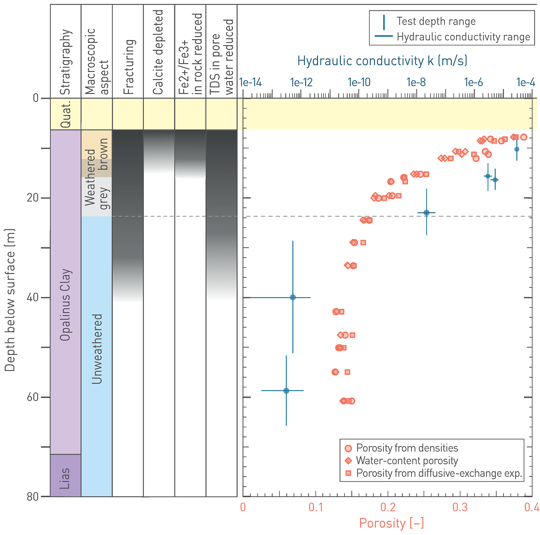
Fig. 6‑46: Rock properties of the Opalinus Clay in the shallow decompaction zone: Synopsis of the observations in the Lausen case study

Figure based on Mazurek et al. (2023b) and Vogt et al. (2017). Dark colours indicate the depth range of alteration. TDS: Total dissolved solids.

Dissolution processes have the potential to alter the hydraulic conductivity of a rock. The host rock and confining units are characterised by varying amounts of clay, quartz and carbonate minerals and by porewaters in thermodynamic equilibrium with these minerals (Section 5.4). Of these, calcite is the most soluble mineral. Groundwaters in the adjacent aquifers are also charac­terised by calcite mineral equilibria (Section 4.5.5, no particular high-pCO₂ waters), that is there is no important driving force for dissolution. Other potentially soluble minerals (rock salt, anhydrite) are not present in either the host rock or confining units²⁰ in significant quantities (Section 5.2). For the Opalinus Clay, dissolution of rock-forming minerals is not considered relevant over the period under consideration, mainly because of the limited amount of soluble minerals and their disseminated distribution (Section 5.4) and because of the very low hydraulic conductivity (Section 5.6).

The upper confining units are generally clay-mineral-rich but include sections with increased carbonate content. The clay-mineral-rich sections are less affected by dissolution processes and will most probably show a similar decompaction behaviour to the host rock. However, for the carbonate-rich sections, decompaction and related carbonate dissolution may result in an increased horizontal permeability. A more pronounced increase in hydraulic conductivity (karsti­fication) may occur if the confining units are uplifted above the relevant local discharge level (~ local baselevel; Section 6.4).

In the provisional disposal areas of all the siting regions, the remaining overburden thickness above the upper confining units is at least 300 m thick in the most likely scenario (Fig. 6‑44), in which no relevant decompaction effects are expected.

An uplift of the upper confining units above the local baselevel is considered very unlikely in NL and ZNO (Fig. 6‑32). For JO, however, fluvial incision of the Aare River may cause lowering of the local erosion base to a level below the top of the Passwang Formation, potentially enhancing carbonate dissolution.

Diffusion properties are closely related to porosity and the pore space architecture (Section 5.8). Porosity depends on overburden thickness (Section 5.2) and consequently also the diffusion pro­perties. However, measurements of the Opalinus Clay porosity in boreholes in Northern Switzerland, where overburden thickness varies between 450 and 1'000 m, indicate only a very weak increase with decreasing overburden thickness (Fig. 5‑10).

The diffusion properties measured in the different TBO boreholes for the Opalinus Clay using tritiated water (HTO) tracers are almost identical (median values differ by less than 4% with no relationship to overburden thickness; Fig. 5‑51). The Opalinus Clay at Mont Terri, where the overburden thickness is less, i.e. ca. 300 m, has an approximately two times higher effective diffusion coefficient (D_e) value compared to the siting regions, which is attributed to the higher porosity at Mont Terri (Section 5.8.3).

A marked porosity-related increase of D_e is to be expected when erosion reduces the thickness of the overburden to a few decametres (Fig. 6‑46). Note that for the transport of anions and cations, D_e is also influenced by the porewater chemistry, which may change slightly over time (Section 6.5.4).

For all the siting regions, the most likely overburden thickness above the provisional disposal areas after the period under consideration (Fig. 6‑44) is a minimum of 400 m, sufficient to prevent an increase in the effective diffusion coefficient D_e in the Opalinus Clay (increase < a factor of ca. 2). The full range of erosion scenarios shows that NL is the most robust with respect to pre­serving this (or even larger) overburden thickness. In JO, this considerably depends on the evolution of the drainage system and associated topography (Section 6.4.4, Fig. 6‑44).

Porewater chemistry of the host rock is a major constraint on radionuclide mobility (speciation, sorption, solubility) and the stability of the engineered barriers. Furthermore, porewater composi­tion affects the diffusion behaviour (Van Loon et al. 2023), with lower salinity (lower ionic strength) leading to lower anion and higher cation diffusion coefficients (Glaus et al. 2024; Section 5.8), the latter mainly for cations undergoing ion exchange reactions.

Porewater constituents can be subdivided into free constituents such as chloride and elements buffered by thermodynamic equilibria with host rock minerals. While the mineralogical com­position can be considered constant over the period under consideration (Section 6.5.6), the free porewater constituents are affected by the diffusive interaction with bounding aquifers. The modelling of the tracer profiles (Section 4.6) shows that the Opalinus Clay porewater may slowly evolve towards lower salinity on a timescale of hundreds of thousands of years. Forward modelling of the Benken dataset suggests a decrease in chloride concentration of less than 1 g/L in the centre of the Opalinus Clay within 1 Myr (see Section 8.6.2 in Nagra 2002). The slowly changing porewater chemistry results in slightly decreasing diffusion coefficients for anions and a slight increase for cations that undergo mainly ion-exchange reactions.

The impact of decreasing porewater salinity on solubility is specific for each radionuclide and depends on the changing ion concentrations. A qualitative comparison of solubilities based on the NL and ZNO reference porewater with the one based on the dilute JO porewater yields only minor differences (Kulik & Miron 2024).

The prerequisites for dissolution processes are the presence of relevant quantities of easily soluble minerals in the rock and circulation of significant quantities of groundwater that is undersaturated with respect to these minerals. Some units below the host rock contain soluble carbonate and evaporite minerals and dissolution phenomena are observed in near-surface positions (Sec­tions 4.5.3.11 and 4.5.3.12). Therefore, the question arises as to whether large-scale dis­solution processes (‘karstification’) at relevant depth could affect the long-term stability of the repository above (Jeannin et al. 2015).

Carbonate dissolution in the Muschelkalk aquifer: Given the position in the sedimentary succession, the relevant zone below the repository will be at significant depth at the end of the period under consideration and certainly below the discharge area of this aquifer. This indicates that the Muschelkalk will not be affected by major decompaction effects and will not be exposed to direct recharge of weakly mineralised waters. Therefore, deep Muschelkalk groundwaters will remain saturated with calcite and near or at saturation with respect to dolomite in the future. That is, there is no or only little driving force for dissolution of the carbonate minerals. Hydrogeo­chemical investigations (Section 4.5.5) evidence a large-scale dedolomitisation process with a reaction progress probably controlled by slow diffusive interaction with the adjacent sulphate-mineral-rich units. In addition, water flow in the Muschelkalk aquifer occurs along a comparably large number of fractures and partly in the porous matrix (Section 4.5.3.12). Overall, there are only negligible to small driving forces for dissolution. Given the nature of water flow and the generally small and limited water fluxes at this depth, the evolution of large cavities is unlikely.

Carbonate dissolution in the Muschelkalk aquifer could also be triggered by cross-formation flow (hypogenic karst development), i.e. caused by groundwater ascending along faults from deeper aquifers such as the Buntsandstein or the crystalline basement. These groundwaters are of different chemical composition, that is they would have some potential to dissolve carbonate minerals. There is evidence for cross-formation flow between the crystalline basement and the Muschelkalk aquifer in structurally highly affected areas related to earlier periods of geological history (Section 4.5.5.5). Within the NL and ZNO siting regions, increasing concentrations of elements such as Li along the flow path (Section 4.5.5.5) indicate mixture with a component that might reside in the matrix of the Muschelkalk aquifer or indicate minor admixture (< ca. 20%) of deeper groundwater along the regional flow path. In contrast, Muschelkalk groundwaters with elevated concentrations of Na and Cl in NL (i.e. Na-Cl type waters) are devoid of particular indications of a basement component (Section 4.5.5.5). In JO, Muschelkalk groundwaters are all of Na-Cl type and may show elevated concentrations of ⁴He and Li (Fig. 4‑114). Here, the Na-Cl type groundwater signature may thus indicate cross-formation flow from deeper units to the Muschelkalk aquifer. Overall, cross-formation flow may occur locally, e.g. along regional fault zones, and cause some dissolution, but this is mostly a subordinate process in the genesis of the deep Muschelkalk groundwaters. In any case, it is a slow process given the residence times of these waters. Cavities of significant size are not expected.

Dissolution of anhydrite (Bänkerjoch Formation) and related loss of barrier function is not expected because of remaining large overburden thickness and self-sealing by anhydrite – gypsum transformation (Section 4.5.3.11). In addition, the groundwaters in the adjacent aquifers are at or near to saturation with respect to the relevant sulphate minerals. In a field study near Stuttgart (Ufrecht 2017), an overburden thickness larger than ca. 40 – 80 m was found sufficient to maintain the original anhydrite component. This agrees with the observations in the Böttstein borehole in Northern Switzerland, where the transformation to gypsum is essentially restricted to less than 60 m depth (data compilation by Mazurek 2017). These observations underline that the Bänker­joch Formation will maintain its aquitard character as long as this minimum overburden is main­tained.

The local salt deposits (halite) in the Zeglingen Formation are also readily soluble. Dissolution is imaginable in the case of direct contact with the strongly halite-undersaturated groundwaters in the aquifers above and below. This might occur, for example, along a transmissive fault con­necting these aquifers. Hydrogeochemical indications for such processes come from the JO area (Section 4.5.5.5) and from the area closer to the Rhine Graben (Waber & Traber 2022). The high Na and Cl concentrations observed in borehole BUL1 are likely explained by a lateral contact with the salt deposit (Section 4.5.5.5). The halite deposits are sandwiched in between anhydrite-rich rocks (including some clay-rich layers), that is these rocks have a self-sealing potential, and the faults are therefore not likely to have high transmissivity (where vertical displacement is small). In any case, the dissolved volume of rock is expected to be small and deformation related to collapse of dissolution cavities is not expected to reach the level of the repository located ca. 300 m above.

Overall, adverse effects due to dissolution below the host rock are considered very unlikely. There are no major drivers for carbonate and anhydrite dissolution. Furthermore, the positioning of the disposal areas takes into account the location of larger faults.

The mineralogical composition of the Opalinus Clay host rock is relevant for the sorption of radionuclides and the buffering of the porewater chemistry. Unaltered host rock also ensures, for example, unaltered diffusion properties (Section 5.8) and hydraulic conductivity (Section 5.6).

A number of studies show that the mineralogical composition of the Opalinus Clay is only altered if the overburden thickness is less than a few decametres (Hekel 1994, Mäder & Mazurek 1998, Mazurek et al. 2023b; Fig. 6‑46).

Given the expected erosion and the remaining overburden thickness (Fig. 6‑44), these processes are not relevant during the period under consideration. The host rock provides a stable and predictable system regarding porewater chemistry, sorption, diffusion properties and hydraulic conductivity.

• Overburden thickness is a determining factor for the long-term hydrogeological evolution of the sites and the ability to maintain the barrier function. A remaining overburden thickness of 200 m is required to ensure efficient self-sealing of fractures in the Opalinus Clay. At the end of the period under consideration, the most likely scenarios at the location of the provisional disposal areas of all sites show at least ~ 400 m of remaining overburden above the host rock. The full range of erosion scenarios shows that NL is the most robust in this regard. In JO, the remaining overburden thickness depends more substantially on the evolution of the drainage system and associated topography.

• Only subordinate changes in diffusion properties of the Opalinus Clay are expected over the period under consideration, related to decreasing overburden thickness or because of changing porewater chemistry.

• Transient effects related to glaciations may affect the geological barrier in terms of pore pressures, hydraulic gradients and advective flux. The impact of these transient processes can be constrained and will result in a short-term but not relevant increase in advective flux out of the Opalinus Clay.

• Aquifers are more strongly affected by long-term evolution, notably the aquifers above the host rock. This mainly affects transport in the aquifers (water fluxes and residence times). Where the aquifers are at greater depth, the effects are smaller or occur later.

• Dissolution processes are not expected to affect the barrier properties of the host rock. This is mainly because the low hydraulic conductivities are maintained, and because the limited amount of soluble (e.g. carbonate) minerals is disseminated within the clay-mineral-rich rock.

• Carbonate-rich sections in the upper confining units are prone to dissolution processes if overburden thickness is substantially reduced and the confining units are located above the groundwater discharge level. This is very unlikely for the NL and ZNO siting regions. JO is least robust in this regard, because fluvial incision of the Aare River may cause lowering of the groundwater discharge level (~ local baselevel) below the level of the Passwang Formation, enhancing the driving forces for carbonate dissolution.

• Dissolution processes below the host rock are unlikely to affect the long-term stability of the host rock because of small driving forces, slow processes and because of an appropriate position of the disposal zones with respect to larger faults.

This section starts with a summary of the long-term geological evolution of Northern Switzerland together with overall conclusions regarding site selection and long-term safety (Section 6.6.1). This is followed by a description of the relevant processes with respect to the anticipated evolution of the landscape around the deep geological repository with the focus on NL (Section 6.6.2).

The general conclusions follow up on the questions posed in Section 6.1.2 for the relevant climatic and erosive processes and their impact on the hydrogeology and geochemistry of the host rock and confining units.

Tectonic evolution

• Tectonic deformation rates in Northern Switzerland are small and are expected to continue to remain small over the next one million years.

• The spatial uplift pattern in Northern Switzerland over the next one million years will continue to be dominated by Alpine uplift. Uplift rates are expected to be < 0.36 mm/yr, most likely ~ 0.15 mm/yr, with relatively small differences between the NL and ZNO siting regions and slightly lower rates near JO.

• Baselevel drop due to subsidence of the Upper Rhine Graben might increase the incision potential of the Hochrhein River and the Aare River. It is expected that sediment supply and ongoing uplift of the Rhenish Massif will compensate for subsidence and work against baselevel drop.

• Inherited faults will localise strain and future deformation. Mainly the regional fault zones will be preferentially reactivated. The location of larger faults is taken into account when planning the locations of the disposal areas.

• If new faults develop in the host rock, they are expected to be segmented and small in length and offset (scaling relationships; see fault architecture in Section 5.5.4).

Climate evolution

• According to different anthropogenic CO₂ scenarios, 3 to 5 large glaciations (LGM-size or larger) are expected that might reach the external Alpine Foreland in the next one million years. The climate conditions during future glacial periods are expected to be similar to those during past cycles.

• Considering present anthropogenic climate change and the longevity of increasing CO₂ levels within the atmosphere, inception of the next glaciation is expected to be significantly delayed, and the next large glaciation may only occur in ~ 200'000 years.

• Each glacial period is expected to be associated with permafrost conditions during the phases of coldest temperatures. Permafrost is expected to reach maximum depths of 100 – 200 m.

• Ice thicknesses and the duration of the ice occupation at the sites varied during past glacial cycles because of the different distances to the Alps and different topography (ZNO > NL > JO). The same pattern will most likely be seen during future glaciations with ice thicknesses between 200 and 400 m and durations of ice occupation between 1'000 and 3'000 years.

• After a glacial state, the climate warms, and climate conditions change from a polar climate (Switzerland largely covered by ice and/or permafrost conditions) towards a continental or temperate climate. Also, a warmer-drier climate cannot be excluded, at least in the high-emission scenarios.

Erosion

• Future erosion processes (glacial and non-glacial) are expected to continue as observed in the Quaternary period, but at lower rates with no major drainage reorganisation, smaller glaciers, delay in glacial inception, and harder-to-erode rocks below the Molasse units.

• The main river system affecting erosion in the siting regions over the next one million years remains the Aare – Rhine River system. The Rhine is further growing at the expense of the Danube with a very limited impact on the incision potential.

• A residual overburden thickness of 200 m classified as reliable for maintaining self-sealing behaviour can be shown for the most likely scenarios in all the siting regions for the period under consideration. Using the 5 – 95% range as a reference, JO shows more limitation for such a 200-m criterion at the location of the provisional disposal area. This site thus depends on the preservation of the local topography (see Fig. 6‑47).

• Excavation of the repository by erosion within the next one million years is extremely unlikely at all three sites. The NL site is most robust in this regard because of the greater repository depth and the expected rates of erosive processes (see Fig. 6‑47).

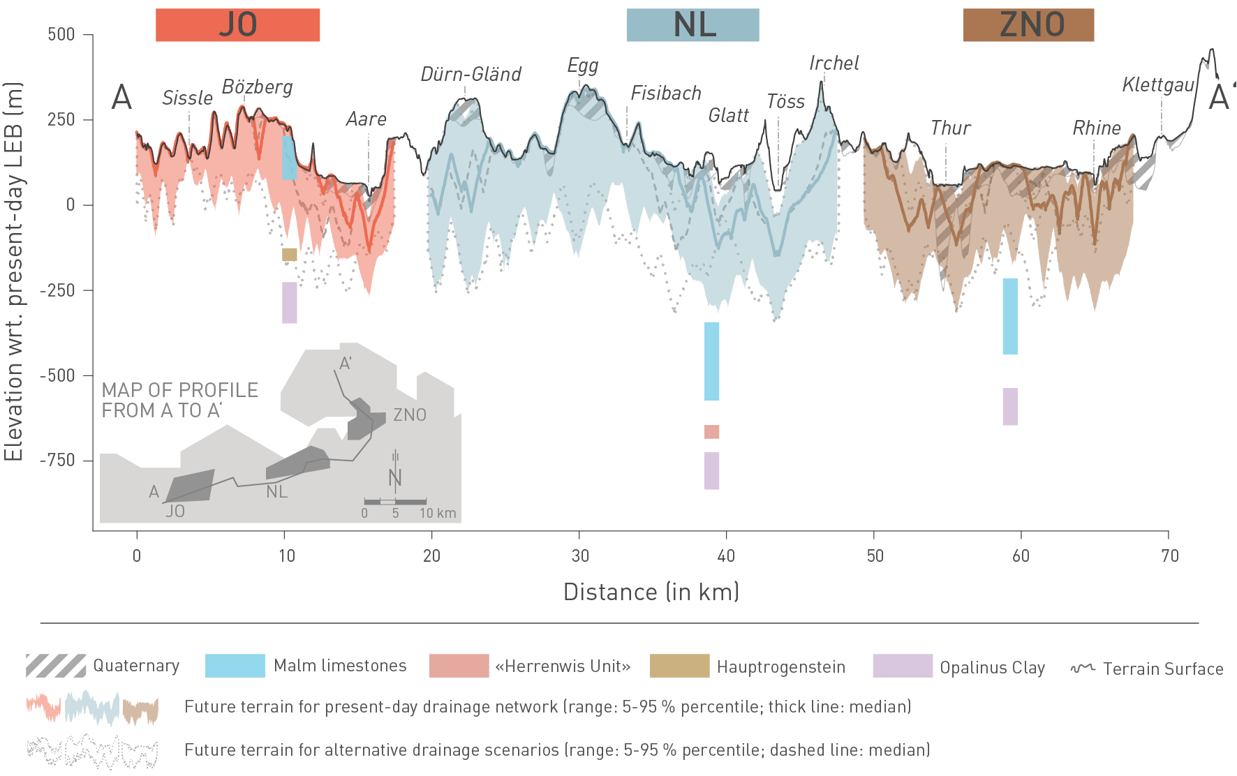
Fig. 6‑47:Synthesis profiles for visualising future non-glacial erosion in the three siting regions

The profile shows ranges of future evolution of the local erosion base and local topography for selected scenarios and selected parameter combinations (see corresponding map repre­sentations in Fig. 6‑35 for the present-day drainage network scenarios and Fig. 6‑37 for the JO alternative drainage scenario Rinikerfeld). The profile location is the same as in Fig. 6‑27. Note that the formation of glacial overdeepenings is not illustrated in this plot. Vertical exaggeration is ~ 20-fold. For the provisional disposal area at JO (lateral position corresponds to the location of lithological column in the plot), the remaining overburden thickness with respect to the coloured and dashed bands of future terrain shown here contributes to the green curve ("Local Topography"; output Model B) in Fig. 6‑44.

Hydrogeology and hydrochemistry

• Deep groundwater flow systems are affected by processes of long-term geological evolution such as large changes in morphology, changing climate or by glaciations inducing high sub­glacial water pressure. This affects discharge paths, water fluxes and residence times in the aquifers. Discharge areas will be progressively located closer to the repository locations.

• Loading and unloading with a few hundred metres of ice will result in minor changes in porosity because of the pre-consolidation of the Opalinus Clay during maximum burial. At the same time, the loading and unloading induces transient over- and underpressures, respectively. The overpressures related to ice loading are of limited magnitude and duration. The overall effect on advective flux in the host rock is thus small to negligible.

• The low hydraulic conductivity of the Opalinus Clay will be maintained over the period under consideration at all sites. This is explained by the remaining overburden thickness of at least 200 m. Depending on the river network evolution, the remaining overburden thickness may be less in JO towards the end of the period under consideration (see above).

• Erosion and decreasing porewater salinity pose minor changes to diffusion properties during the next one million years.

• Dissolution processes are not expected to affect the barrier properties of the host rock and confining units in a significant way.

• Overall, the host rock and confining units provide a stable and predictable environment for hosting the repository. The deepest site, NL, is most robust in this regard.

In the following, we summarise the expected long-term geological evolution²¹ of the NL siting region over the next one million years. This geological storyboard supports the discussion on the repository evolution in Nagra (2024p).

Long-term rock uplift, fluvial incision and remaining overburden thickness

The Rhine will grow at the expense of the Danube, by headward erosion rather than through major river capture events. The evolution of the river profile will be largely controlled by rock uplift and sediment input. The bedrock erodibility will only be of secondary importance for vertical fluvial incision but might have an influence on lateral erosion.

The spatial pattern of rock uplift in Northern Switzerland over the next million years will continue to be dominated by Alpine uplift, regardless of whether it is a matter of tectonic uplift or isostatic compensatory movements. In simplified terms, the main uplift gradient can be assumed to cause increasingly higher rates from the external foreland basin towards the Alps along a direction that is approximately perpendicular to the Alpine chain. The long-term rates are low. Total uplift of ~ 170 m (between ~ 25 m and a maximum of ~ 360 m [5 – 95%]) over a million years is assumed for the NL siting region. Short phases of significantly higher rates might be associated with glaci­ations of extensive foreland glaciations (Fig. 6‑48). This in turn may cause temporarily enhanced fluvial incision (after backfilling of perialpine lakes).

Over long time periods, incision rates are generally expected to be in the same range as uplift rates. Significantly greater incision can only be achieved by additionally lowering the regional baselevel. As long as the Rhenish Massif continues to be uplifted, this location (approx. near Bingen; see Fig. 6‑5) decouples the Upper Rhine (and thus the Hochrhein) from the sea. The sedimentary basin of the Upper Rhine south of Bingen is controlled by tectonic subsidence and sediment input at the transition to the Hochrhein near the city of Basel. Today, there is no disturbance of the river profile at this point; the subsidence is roughly compensated for by sedi­ment accumulation. This sedimentation might be additionally linked to a buffer effect associated with the low-subsidence area of the Karlsruhe Swell. Potential elevation gain by short-term over­supply of sediment is compensated for over the long term by vertical incision into these sediments. Averaged over the next million years, however, it is considered possible that the baselevel at Basel might fluctuate by up to ± 70 m.

Under these boundary conditions, a vertical fluvial incision of ~ 160 m is most likely (between 80 and 380 m [5 – 95%]) at the confluence of the Aare and Rhine, i.e. near NL (see Fig. 6‑48). This is in good agreement with Quaternary incision on a million-year timescale around the area of NL. Given these incision estimates, a remaining overburden thickness of ~ 550 m (350 – 670 m [5 – 95%]) can be expected, potentially increased by future evolution of local topography.

Given these constraints, it is therefore expected that the future groundwater discharge area will be located progressively closer to the position of the provisional disposal area. The flow path will be shortened compared to today and incipient decompaction affecting the Malm aquifer due to erosional unloading may then increase hydraulic conductivity. A more active flow system will develop, although this happens only late in the period under consideration. Importantly, the remaining overburden thickness is sufficient to avoid any decompaction effects or to affect the self-sealing capacity of the host rock and the clay-rich confining units. The upper confining units will stay well below the local erosion base, preventing dissolution of carbonate-rich sections. The host rock provides a stable and predictable system in terms of porewater chemistry, sorption, diffusion properties and hydraulic conductivity.

Because of the significant remaining overburden, the aquifers below the host rock will experience negligible changes in their properties. The Muschelkalk aquifer will not be affected by decom­paction effects and will not be exposed to direct recharge of weakly mineralised waters. There­fore, deep Muschelkalk groundwaters will remain saturated with calcite and near or at saturation with respect to dolomite in the future, preventing significant dissolution of the carbonate minerals below the provisional disposal area.

Short-term modulation of fluvial incision by glacial/interglacial cycles

Long-term incision will be modulated by phases of sediment accumulation with no net vertical incision. The sediment dynamics will be largely controlled by glacial/interglacial cycles. During the interglacial warm periods, a relatively high precipitation rate is expected and consequently a relatively high water discharge. At the same time, the sediment flux may be limited by a weak coupling between the glacially conditioned sediment sources and the rivers. During a renewed Alpine glaciation, the reworking of periglacial deposits by the advancing glaciers and an increase in the area subject to subglacial erosion should lead to a peak in sediment flux. During the main glacial phase, sediment flux is assumed to be larger than the interglacial rate because of increased glacial activity, sediment generation in adjacent permafrost terrains and the effect of greater climate variability. At the termination of glacial conditions, a peak is inferred in water discharge because of the warming-induced increase in atmospheric moisture and a pulse of meltwater from the retreating ice. The greater water availability induces faster glacial sliding and hence an increase in glacial erosion. In combination with the paraglacial adjustment of the landscape, this should result in a maximum contribution of sediment to the fluvial system. However, after glacial retreat, the sediment is trapped in perialpine lakes and overdeepened basins for up to several tens of thousands of years, thus reaching into the interglacial period.

The expected glacial scenario and deep glacial erosion

According to different anthropogenic CO₂ scenarios, 3 to 5 large glaciations (LGM-size or larger) might reach the Alpine Foreland in the next one million years. The next glacial inception will be significantly delayed, and the next large glaciation will only occur after the next ~ 200'000 years (Fig. 6‑48). During extensive future foreland glaciations, deep glacial erosion may take place in the eastern part of the NL siting region, where present-day relief is low. This area could be repeatedly glaciated if future glaciers are of similar or larger extent as the penultimate glaciation (Beringen). Maximum ice thickness is estimated at 400 m and a duration of the ice coverage of a few thousand years.

Total cumulative erosion depth in such a case is is most likely to reach ~ 70 m below the local erosion base (30 – 360 m [5 – 95%]). Because the baselevel has already been lowered, deep glacial erosion could reach the Malm limestone late in the period under consideration. It is expected that the Malm limestone is on average only half as erodible as the Molasse-type rocks in Northern Switzerland. It is thus highly unlikely that glacial overdeepening will reach the host rock.

During cold climate periods, the hydrogeological conditions will be affected by glaciation.

An increase in hydraulic gradient is possible during large foreland glaciations but will be limited in magnitude and with a comparably short duration. The overall effect on advective flow in the host rock during these glaciations is small to negligible. The additional ice load can result in an increase in hydraulic head in the Opalinus Clay relative to the confining units with changing direction of the hydraulic gradient between glaciation and glacial retreat. The temporary increase in advective flux because of glacial loading is considered insignificant.

Occurrence of deep-reaching permafrost

Each glacial period is expected to be associated with permafrost conditions during the phases of coldest temperatures. This timing does not necessarily correspond to the timing of the glacial maximum but might pre- or postdate this peak (Fig. 6‑48). Depending on the glacial scenario, such behaviour may be expected initially after 200'000 years. During coldest temperatures, deep-reaching permafrost might affect the flow systems in deep aquifers mainly in terms of reducing water fluxes and increasing residence times. Permafrost is expected to reach maximum depths of 100 – 200 m.

Because of a lower limit of remaining overburden above Top Opalinus Clay of ~ 300 m, the expected maximum depth of 200 m permafrost does not challenge the barrier integrity of the host rock by freeze-and-thaw effects.

Earthquakes and faulting

The site is located within a low-seismicity intraplate domain. Faulting is primarily related to shortening in the Alps and in the Internal Jura, as well as transtensional deformation within the Upper Rhine Graben and the Hegau – Bodensee Graben. Current plate dynamic forces define the stress field that is predicted not to vary significantly from the present direction. Rates of strain accumulation are anticipated to be low over the next one million years.

As typical for intraplate areas, the location of faulting is expected to change over time, and areas currently seismically inactive might become the focus of future seismic activity. Earthquakes and fault ruptures are thus possible in the vicinity of the siting regions. Accordingly, changes in local stress conditions might trigger faulting. Such changes might be applied by vertical glacial loading or unloading, large erosion events, or by loading from interaction with neighbouring faults (Fig. 6‑48). Importantly, irrespective of timing and trigger, significant offsets may occur along existing larger faults and not along subseismic faults or as a result of new fault creation. Such regional fault zones bound the siting region and will be considered when positioning the disposal areas. Subseismic faults and potential new faults in the Opalinus Clay are expected to be seg­mented and short in length and offset. Relevant changes of the barrier effect by future earthquakes and faulting are thus not expected.

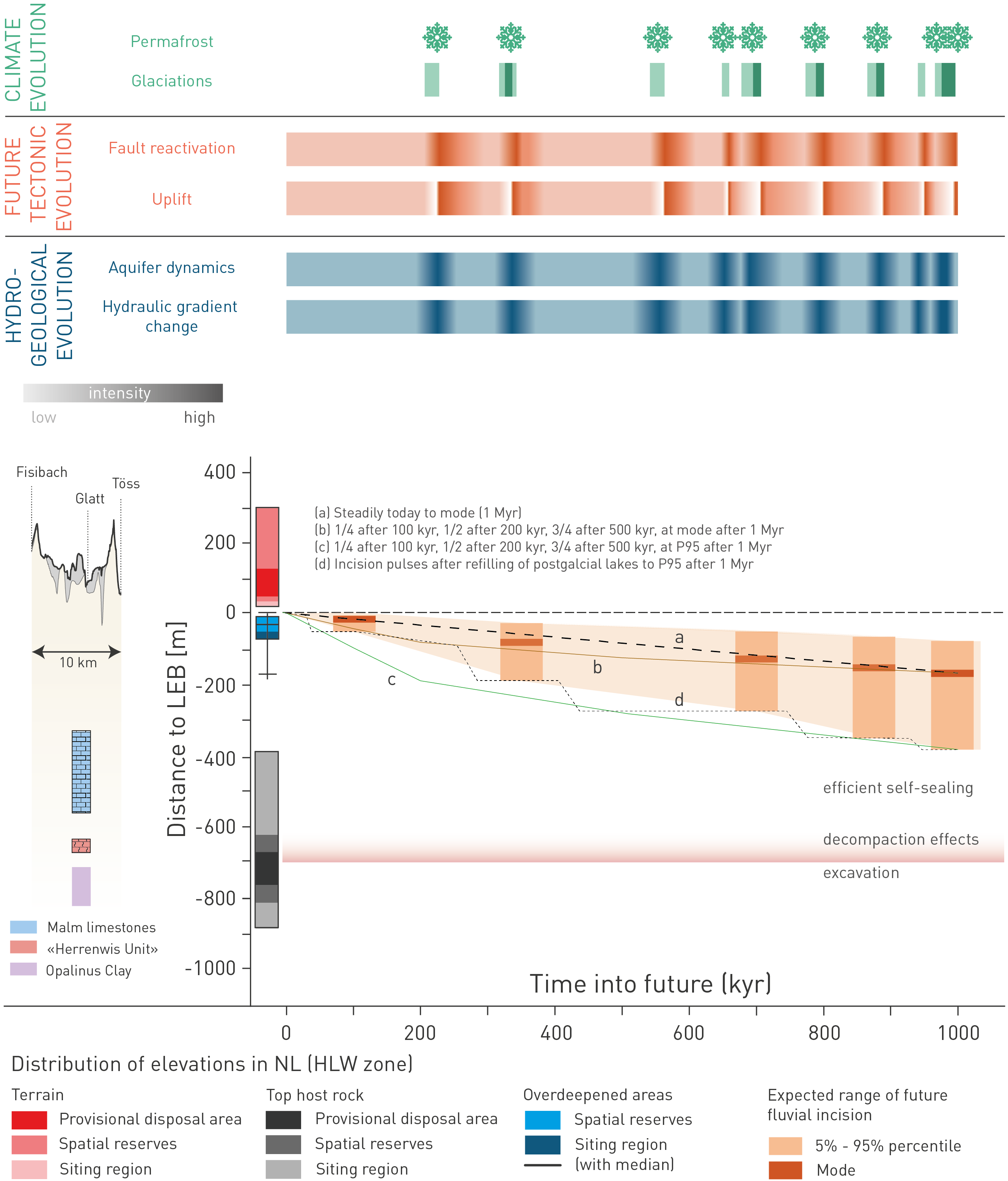
Fig. 6‑48: Schematic diagram summarising the long-term geological evolution of the NL site

The diagram summarises the elements that describe the expected long-term geological evolu­tion over the next one million years for the NL site. The panel on the left-hand side shows the present-day site-specific constraints extracted from the cross-section in Fig. 6‑27 between Fisibach and Töss and a simplified depth profile with boxplots highlighting the distributions of host rock, local topography and glacial overdeepenings within the siting region, the spatial reserves and the location of the provisional disposal area. The local erosion base (LEB) con­stitutes the reference for the depicted present-day elevations and the future evolution. As a result of long-term rock uplift, modified by transient climate effects, the local erosion base will be lowered by fluvial incision (orange boxes in panel on right-hand side, see mode for the most likely values of fluvial incision). Potential incision pathways are possible during the one million years (e.g. a or b), others are less likely but shown nevertheless because they provide potential calculation cases to show the robustness of the site safety (e.g. c and d). Phases of glacial erosion with potential overdeepening are also highlighted in this upper right panel. Such phases of glacial erosion are coupled to large future foreland glaciations, as depicted by the dark-green bars in the panel "Climate evolution". Note that glacial over­deepening is not shown in the erosion plot below (see Fig. 6‑44 for full remaining over­burden, including glacial overdeepening). Glacial conditions and permafrost, how­ever, are expected to occur in semi-regular intervals. The timings delineated here correspond to the 500 PgC scenario of future climate models. The panel "Future tectonic evolution" also high­lights a certain synchronicity with future glaciations. For instance, this can be pulses of increased rock uplift after deglaciation (rebound) or phases of enhanced fault activity by reactivation from static stress changes. In general, however, fault reactivation along pre-existing structures might occur at any time within the one million years, and the increased rock uplift is expected to balance out over the long time period. The climate and tectonic triggers may alter the hydrogeological conditions (blue bottom panel). Accordingly, such changes might occur synchronously with the phases at and shortly after glaciations.