Future evolution of the local erosion base

The analysis of future fluvial incision of the Hochrhein (i.e. approximately between the cities of between Stein am Rhein and Basel) and thus lowering of the local erosion base is based on the stream power incision model (SPIM) (for more detail see Nagra 2024k). The SPIM is frequently used in landscape evolution models that include tectonic uplift U. The main advantage is the low model complexity and its relatively straightforward numerical implementation, which allows its application to long timescales (10⁵ – 10⁶ years) and to investigate different boundary conditions. According to the SPIM, the rate at which rivers incise is a function of the drainage area A and channel slope S = dz/dx raised to the power exponents m and n, respectively, and multiplied by a bulk parameter K which is a dimensional coefficient of erosion often simply termed erosional efficiency or erodibility coefficient (for more detail see Nagra 2024k).

When addressing the future, it is expected that parameters such as rock uplift U (Section 6.2.2), erodibility coefficient K or upstream drainage area A might change over time. Consequently, the evolution of the intermediate baselevel at the transition from the Alpine Foreland to the Upper Rhine Graben near Basel needs to be considered (Section 6.2.2). These parameters were elicited independently as subjective probabilities (see Fig. 6‑29: Model A, Section 6.4.2.3 and Nagra 2024k).

Rock uplift

Spatial rock uplift is approximated here by a plane, i.e. rock uplift is modelled as a linear function of longitude and latitude. The main assumption is that the Alpine uplift provides the dominant cause for the geometry of the uplift plane. In simplified terms, the main gradient causes higher rates from the external foreland towards the Alps along a direction that is roughly perpendicular to the Alpine chain. However, the plane is based on the uncertain parameters of rock-uplift rate at one position (here Brugg), the gradient at which uplift is rising, and the azimuth direction along which the gradient is applied (see Nagra 2024k for more information). Based on the plane, cal­culated from these elicited parameter distributions, the uplift can be evaluated for any coordinate within the investigated area, for instance, for the locations of the siting regions (Fig. 6‑30, Tab. 6‑1). Note the higher rates for the shorter time frame of 100'000 years that includes similar values as measured using geodetic methods (Section 6.2.2).

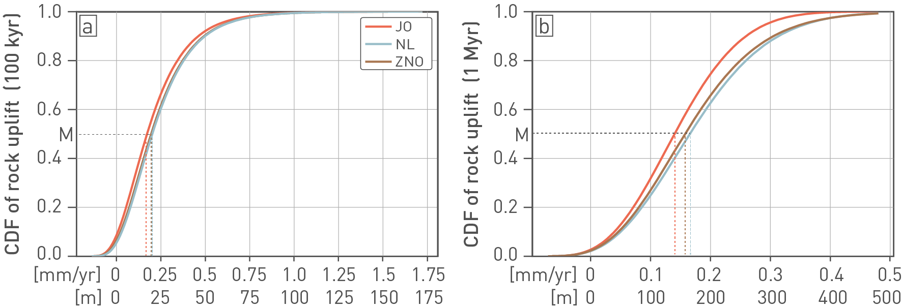
Fig. 6‑30:Inferred future rock uplift rates in the three siting regions over the next 100'000 and one million years

Rock uplift rate is defined as the total rate of bedrock uplift in mm/yr that is expected as a response to tectonic processes and as an isostatic response to loading or unloading, including the response to loss of ice cover. The reference level for rock uplift is the geoid. The estimates are based on the assumption of a planar uplift pattern caused primarily by Alpine uplift. The results are calculated for the location of the provisional disposal areas and shown as cumula­tive distribution function (CDF), where the value of 1.0 (y-axis) equals to 100% cumulative probability. The letter M at both y-scales refers to the median value, i.e. the 50% quantile (value 0.5). The corresponding median values can be read at the x-axes (compare Tab. 6‑1). (a) CDF of estimates for the time frame of 100'000 years. (b) CDF of estimates for one million years. Note that the shorter time frame of 100'000 years allows higher rates (see Nagra 2024k for more details). The lower x-axis translates the rates to cumulative amount of rock uplift for the respective time frames.

Tab. 6‑1:Inferred future rock uplift rates

Rates are estimated at the locations of the provisional disposal areas of the siting regions for 100'000 and one million years, respectively (see Fig. 6‑30). The location of the provisional disposal area is shown in Fig. 6‑34. Values are rounded to the second digit. The 5 – 95% of the total probabilities are considered the expected range in this assessment

Erodibility coefficient

The rock types of Northern Switzerland comprise a variety of assumed resistance against erosion. They were divided into four erodibility classes (EC) based on lithological considerations and the lithostratigraphic units differentiated in the 3D geological model "Nagra Regionalmodell 2012" (Gmünder et al.. The classes comprise EC 1 = Quaternary unconsolidated sediments, EC 2 = Bedrock Class "soft", EC 3 = Bedrock Class "medium", and EC 4 = Bedrock Class "hard" (Fig. 6‑21). It is generally assumed that the classification of erodibility follows the trend of EC 1 > EC 2 > EC 3 > EC 4. This allows distributions to be assigned for the erodibility coefficient (Kvalues) needed for modelling fluvial incision and later local topography (see Section 6.4.3.2) using the SPIM equations.

The geological map of Northern Switzerland 1:100'000 (Isler et al. 1984) was first used to map spatially variable values of the erodibility coefficient K (depending on rock type) on the present-day topography, focusing on the JO siting region and surrounding area (Graf 2022). This first-order assessment was done by extracting ranges of apparent K values from the present-day land­scape based on drainage area and gradient along the channel network. Lithological mapping along the Hochrhein is less distinct than within the 3D geological model. Here, rock types of EC 2 and EC 3 were combined into one class (here ECb) of weak to intermediate resistance to erosion (see Nagra 2024k for more detail).

Importantly, an uplift value of 0.1 mm/yr was spatially uniformly applied to the area used for the K mapping (Graf 2022). Simplified, this means it was assumed that the present-day landscape has evolved under a background rock uplift rate of 0.1 mm/a. Under the chosen SPIM assumption (n = 1, m = 0.45; Nagra 2024k), uplift and K values scale linearly. Accordingly, the elicited distributions for the K values of the four erodibility classes included ranges that were scaled to include variability in the uplift value. These ranges are consistent with the previously elicited one million years RIO distribution for uplift at Brugg (UBR, see above and Nagra 2024k for more detail).

The elicitation followed a rather pragmatic, systematic procedure. First, the general assumption was that the median value of each erodibility class, which was derived by the landscape inversion (Graf 2022), reflects the most robust K value of the respective class. The uncertainty distribution around this value should then reflect the scatter (excluding artefacts originating from low gradients at plateau areas or within flood plains). It should also be accounted for transient effects from spatially non-uniform uplift or incision within the landscape and for the uncertainty caused by the uplift assumption of 0.1 mm/yr (see above).

The mean values of the elicited parameter distributions vary by a factor ~ 1.5 and follow the pattern EC 1 > EC 2 > EC 3 > EC 4. The variability of Kvalues within a distribution can be in the order of one magnitude (see Nagra 2024k).

Baselevel changes

In addition, to account for the downstream change from the tectonic domain of the Alpine Fore­land into the subsiding domain of the Upper Rhine Graben, the parameter baselevel drop (BL) was introduced and elicited (Fig. 6‑31). Baselevel in this context is considered with respect to sea level. Here, negative values reflect net baselevel gain. Accordingly, baselevel gain would mainly correspond to sediment accumulation, while baselevel drop can be both rock subsidence, which is not balanced by sedimentation, or incision into the present Quaternary fill.

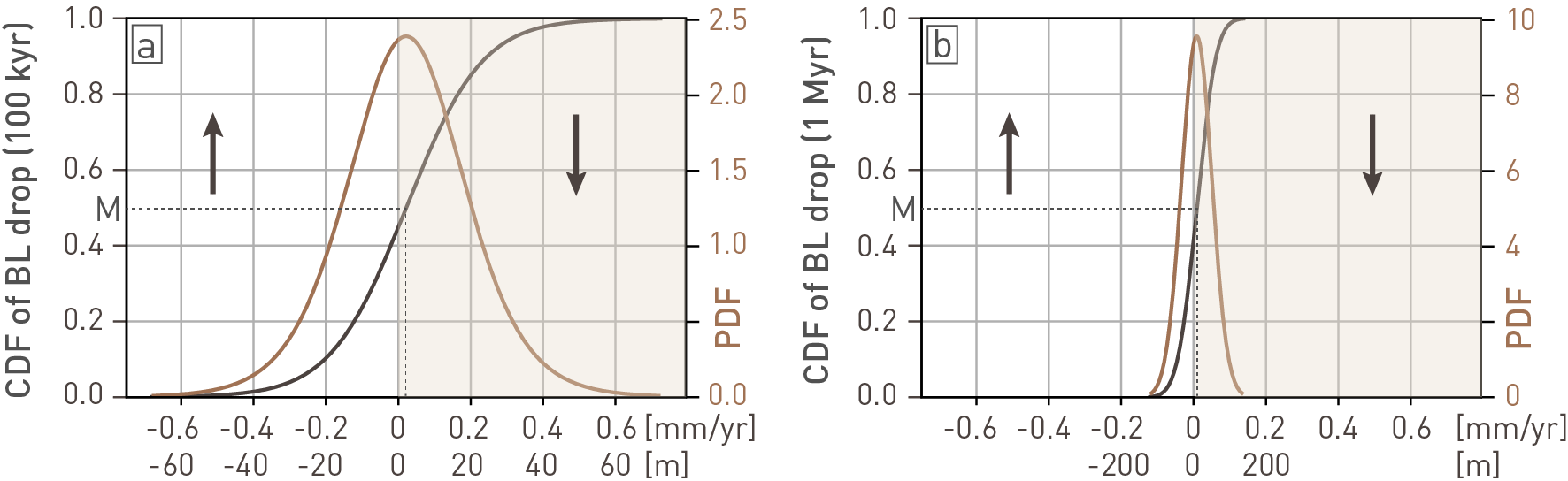
Fig. 6‑31:Total assumed probabilities for baselevel drop downstream of Basel

The total assumed probabilities of the rate of baselevel drop are based on expert judgement (see Nagra 2024k). Probabilities are shown as cumulative distribution function (CDF, see caption of Fig. 6‑30 for explanation) and as probability density function (PDF, brown colour). PDF visualisations allow to assess the most probable values, which are identified by the bulge of the curve (here close to 0 mm/yr). In contrast, lowest probabilities are reflected in the tails (a) 100'000-yr time window and (b) one-million-year time window. Negative values correspond to net baselevel gain. For both time frames, the baselevel downstream of Basel is expected to be stable with a very slight tendency towards baselevel drop. The letter M reflects the median value. The lower x-axis translates the rates to cumulative amount of baselevel change after the respective period under consideration, i.e. 100'000 yr in (a) and one million yr in (b). Note the similar x-axis to highlight the higher rates allowed during shorter periods.

Based on the present-day longitudinal profile and terrace distribution in the Hochrhein and near Basel (Fig. 6‑19 and Fig. 6‑20), the baselevel downstream of Basel is expected to be stable with a very slight tendency towards baselevel drop. However, fluctuations in the order of ~ 30 m (5 – 95%) within the next 100'000 years and up to ~ 60 m gain and ~ 80 m drop (5 – 95%) after one million years appear to be possible in light of the future dynamics of the Upper Rhine Graben and Rhenish Massif (Section 6.2.2) as well as climate-driven sediment flux (Sections 6.3.1 and 6.4.1.2) and were thus included in the uncertainty estimates for future fluvial incision. A baselevel gain of ~ 30 m would roughly reflect the thickness of the Niederterrasse deposits at the location around Basel. Allowing for an additional sediment pulse (e.g. after filling of the Bodensee and Zürichsee), such sediment accumulation seems to be a plausible scenario for a time span of 100'000 years. Yet another plausible scenario would be that, after filling of these peri-Alpine lakes, the sediment pulse fails to appear because of a prolonged interglacial and exhausted sedi­ment sources in the catchments (see Section 6.3.3.1). In such a case, incision into the fill as seen today in large parts of the Hochrhein and Upper Rhine Graben could be expected to continue. Such a scenario could cause net baselevel drop down to the base of the Niederterrasse deposits. Higher fluctuations are allowed in the million-year time window, as it is more likely that larger glaciations will occur (Sections 6.3.3.1 and 6.4.3.3) and supply large amounts of sediment. A baselevel gain of no more than the approximate difference between the top of the Hochterrasse deposits and the river surface and a baselevel drop of approximately half the elevation difference between Bingen and Basel were considered as reasonable assumptions. This estimate is based on the assumption of continued rock uplift of the Rhenish Massif and preservation of the intermediate baselevel near the city of Bingen (see Section 6.2.2).

Changes in drainage area

Based on geometric considerations of the fluvial landscape (Section 6.4.1.2), far-reaching effects influencing the drainage system of Aare and Rhine, similar to those experienced during Pliocene-Quaternary times, are not to be expected at this location for the next million years. A larger piracy scenario that would theoretically be possible late in the period under consideration considers the capture and diversion of the Iller River. Simulations show that such a scenario does not have a major impact on discharge and the vertical erosion potential of the Hochrhein (see Nagra 2024k for more detail). Yet another scenario considers the future increase of the Rhine discharge at the expense of the Danube via karst sinkholes along the Danube. However, even with the full incorporation of the upper Danube catchment into the Rhine catchment, this increase makes only a minor contribution to the fluvial erosion and the longitudinal river profile evolution in the Hochrhein for the next one million years (Nagra 2024k).

Another reasonable scenario would be the diversion and shortcut of the Alpenrhein across a few metre high swell at Sargans, subsequently following a path through the Walensee.

While the Rhine catchment in the area of the siting regions grows at the expense of the Danube, it might lose area towards the Rhone River within the westernmost reaches east of Lac Léman. Headward erosion might capture the Upper Aare, e.g. in the area west of Yverdon (Fig. 6‑19a, see also Nagra 2014c, Dossier III). Such a scenario could cause a baselevel drop with further headward erosion because the Rhone River with ~ 800 km length is significantly shorter than the Rhine River. However, it is not expected that headward erosion would reach the Hochrhein area within the period under consideration. Instead, the loss of Aare catchment would considerably reduce the incision potential of the Hochrhein.

Using a variety of scenarios for changes in future discharge/catchment, as mentioned above (capture of Iller, capture of Upper Danube, diversion of Upper Aare towards west, and diversion of the Alpenrhein across the swell of Sargans) that are ranked by their plausibility, and variants for the parameters based on expert degree of belief, SPIM was used in a Monte Carlo environment to generate probable future river profiles between the outflow of the Bodensee and Basel (i.e. the Hochrhein) at time T^x (100'000 years and one million years) from all parameter combinations (see Nagra 2024k for more detail).

Modelling results

The results are visualised in Fig. 6‑32a for incision after 100'000 years and Fig. 6‑32c for incision after one million years. The left panel shows the realisations of future longitudinal Hochrhein profiles in grey with the present-day river profile (in blue) and the elevations of Bingen and sea level as reference regional baselevels. The darker the future river profiles appear, the more likely is the amount of incision at this position. Baselevel gain flattens the profiles, while baselevel drop allows stronger incision. Because of the more proximal position with respect to the intermediate baselevel in Basel, this influence is largest within the area of JO. The orange boxplots in Fig. 6‑32a and c describe the uncertainty distributions of the rock uplift that the provisional dis­posal areas (circles) might undergo during the same respective time. Using these distributions of rock uplift and future incision, the remaining overburden thickness above the repository location with respect to the local erosion base can be determined (Fig. 6‑32b and d). In these plots, the boxes correspond to specific quantiles (see legend) and the violins reflect the distributions, such that the range of the violins extends past the extreme data points. The bulge corresponds to the most likely values.

The SPIM simulations using all parameter combinations show that fluvial incision itself is not expected to present any threat to the barrier function at ZNO and even less at NL. However, they reveal a considerable number of scenarios in which the repository in JO would be uplifted to, or even above, the future local erosion base (i.e. at the position of the Sissle outlet) after one million years (Fig. 6‑32d). JO would need to rely on the preservation of the additional topography situated above the local erosion base. The results of simulations of the evolution of this local topography are discussed in the next section (Section 6.4.3.2).

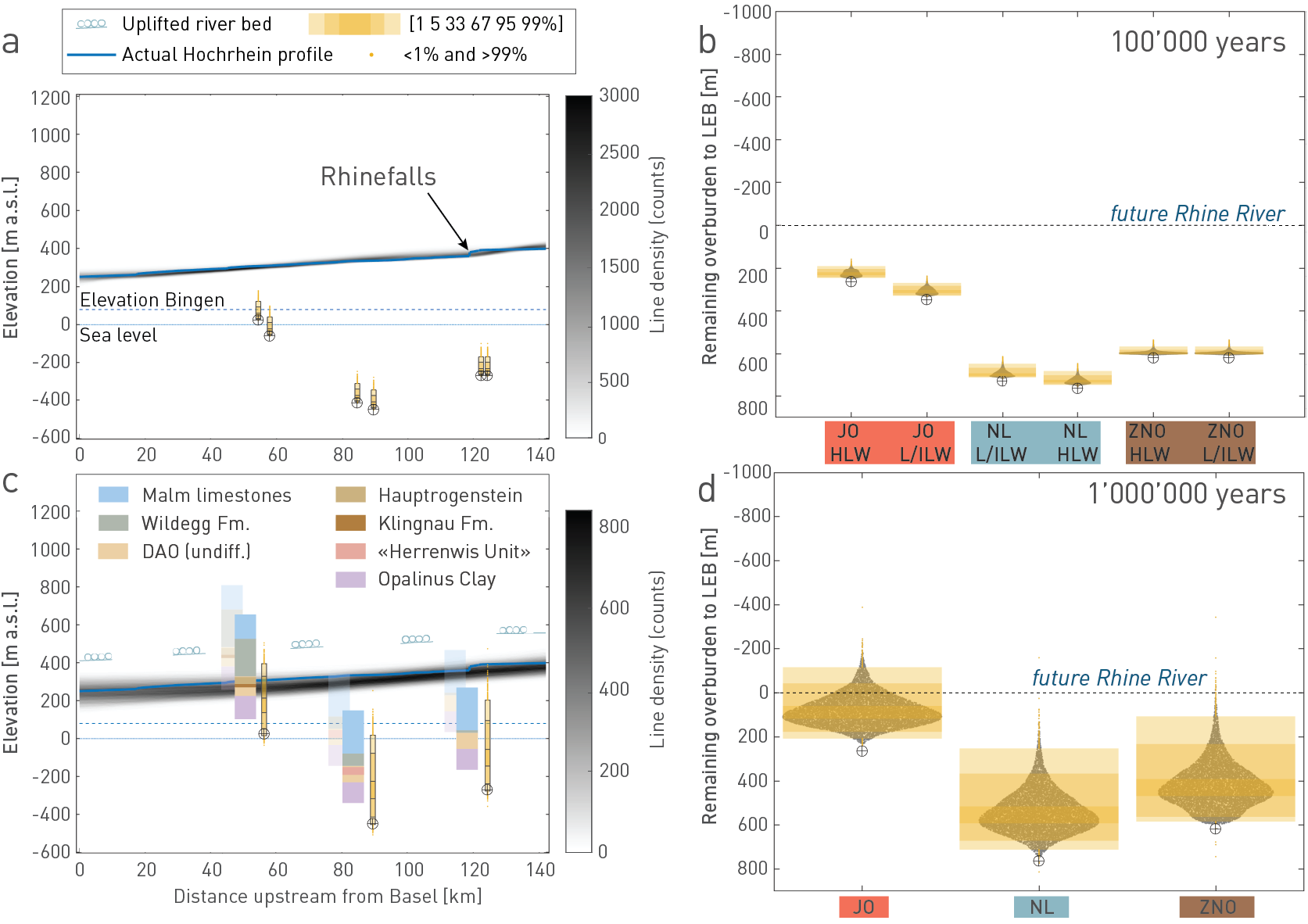
Fig. 6‑32:Results of fluvial incision modelling using the Stream Power Incision Model (SPIM)

The left panel shows the realisations of future longitudinal Hochrhein profiles in grey for 100'000 years (a) and for one million years (c). Also shown are the present-day river profiles (in blue) and the elevations of Bingen and sea level as reference baselevels. The circles correspond to the depth of the provisional disposal areas at the time of emplacement. The orange boxplots above the circles describe the uncertainty distributions of the rock uplift that the disposal areas might undergo in these times. As an example, the stratigraphic columns at the locations of the provisional disposal areas are uplifted according to the median and the 95^th percentile (transparent) – highlighting which units might be incised after one million years, if the Hochrhein or another main river were to flow directly across the disposal area by that time. Also shown are symbolised gravel deposits assuming they were also uplifted uniformly according to the median uplift value (and subsequently incised equally along the profile). As such, they represent the present-day riverbed that becomes remnants of a future terrace surface. The remaining overburden thickness above the repository with respect to the local erosion base is shown in the right panel for 100'000 years (b) and one million years (d). Note that these distributions are calculated for downstream positions along the Hochrhein (i.e. the Sissle confluence for JO, the Aare confluence for NL, and the Thur confluence for ZNO, see Fig. 6‑29). DAO: Dogger Group above Opalinus Clay.