
Simulations of past climates (Section 6.3.1) are used to gain a better understanding of the potential development of glaciers in the Alps, with special focus on the northern central Alps and corresponding ice flow into the forelands of Northern Switzerland and adjacent Southern Germany. The climate simulations of PI, MIS 2, MIS 4, MIS 6, MIS 8 and MIS 16 and a climate signal proxy are combined to construct a transient climate over past glacial periods. This transient climate is used to force thermo-mechanically coupled, three-dimensional transient ice-flow models to simulate the dynamic evolution and basal conditions of glaciers in the Alps (see Nagra 2024j for further details).
The coupled climate and glacier modelling is used to assess the effects of ice-flow dynamics and related erosion potential in the siting regions during previous glacials. The assessment is based on quantitative criteria that incorporate the physical processes upon which glacial erosion depends (e.g. ice thickness, timing and duration of ice occupation, basal ice temperature, basal sliding velocity and subglacial routing of meltwater). These criteria can be derived from the numerical reconstruction of the ice surface geometry (see Fig. 6‑14), flow dynamics and temperature field of the Alpine Ice Field and, in particular, the Rhine Glacier system (Fig. 6‑16) during past glaciations.
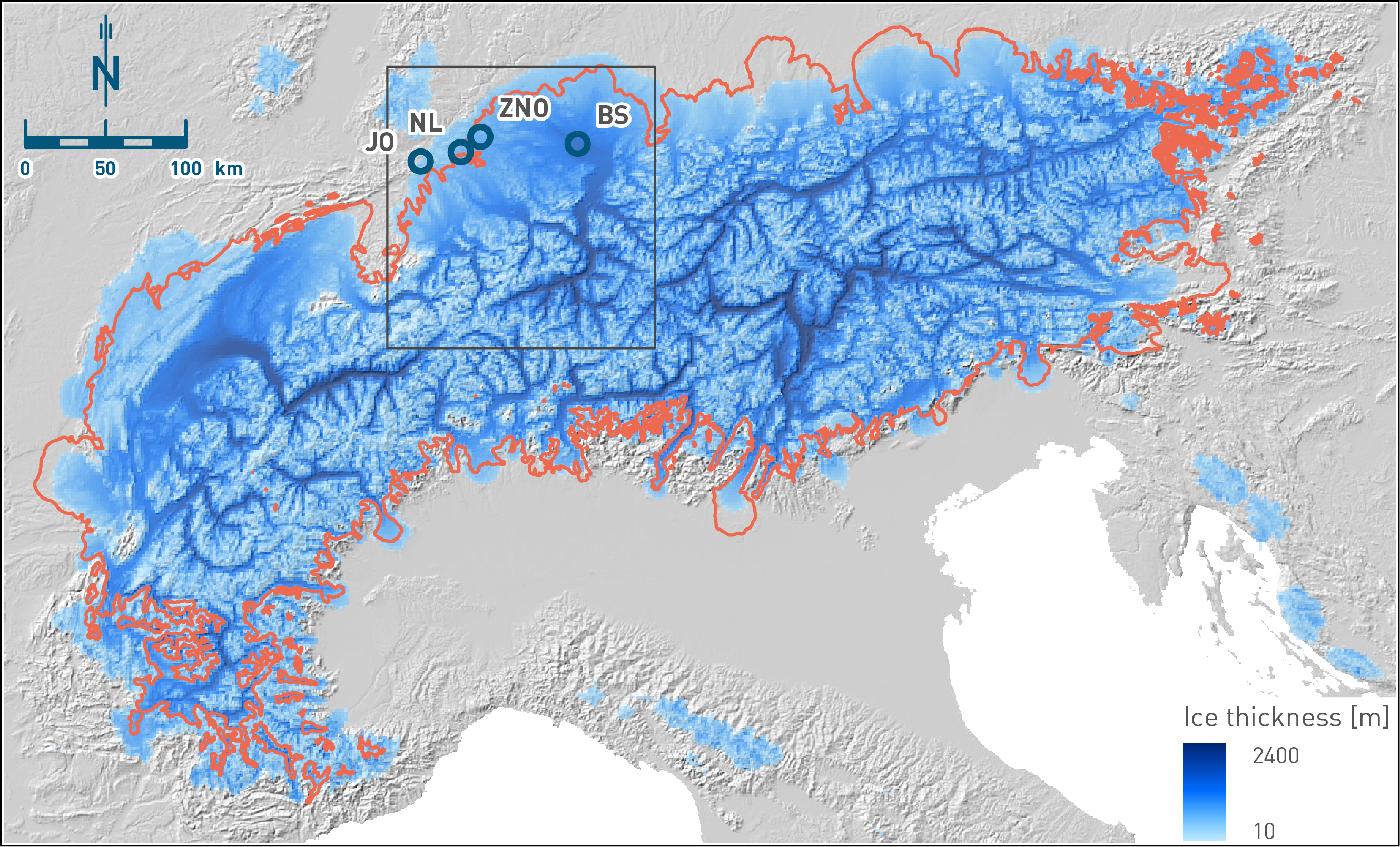
Fig. 6‑14:Modelled maximum ice thickness and extent of the Alpine Ice Field during MIS 2
Geomorphologically reconstructed LGM outline is modified after Ehlers et al. (2011) (red line). Note that different glacier lobes reached their maximum ice thicknesses and extents at different times because fluctuations are controlled by the size of catchments and the resulting inertia of each glacier. The blue circles (JO = Jura Ost, NL = Nördlich Lägern, ZNO = Zürich Nordost, BS = Bodensee) indicate locations where ice thickness and duration of ice occupation have been evaluated (Fig. 6‑15). The box shows the Rhine Glacier system (outline of Fig. 6‑16). As basal topography for the model simulations, the publicly available NASA Shuttle Radar Topographic Mission (SRTM, http://srtm.csi.cigar.org/), the Digital Elevation Model (DEM), re‑sampled at 2 km resolution and with major lakes and present-day glaciers removed (Farinotti et al. 2019) are used.
The modelled maximum east to west extent of the Alpine Ice Field during the LGM matches the geomorphological reconstruction of Ehlers et al. (2011) fairly well (Fig. 6‑14Fig. 6‑19). Furthermore, the results show that the flow dynamics of individual modelled glaciers agrees with several independent key geological observations, including moraine-based maximum reconstructed glacial extents, known ice transfluences and trajectories of erratic boulders of known origin and deposition (Jouvet et al. 2023).
The boxplots in Fig. 6‑15 show the results from different simulations that were carried out as part of a sensitivity study (Nagra 2024j) and suggest a maximum ice thickness of ~ 200 – 400 m and a duration of ice occupation of ~ 1'000 – 3'000 yr in the ZNO and NL siting regions, while JO essentially remained ice-free. Ice thickness and ice occupation duration are significantly larger in the Bodensee region (BS in Fig. 6‑15) due to its more proximal position to the Alpine front.
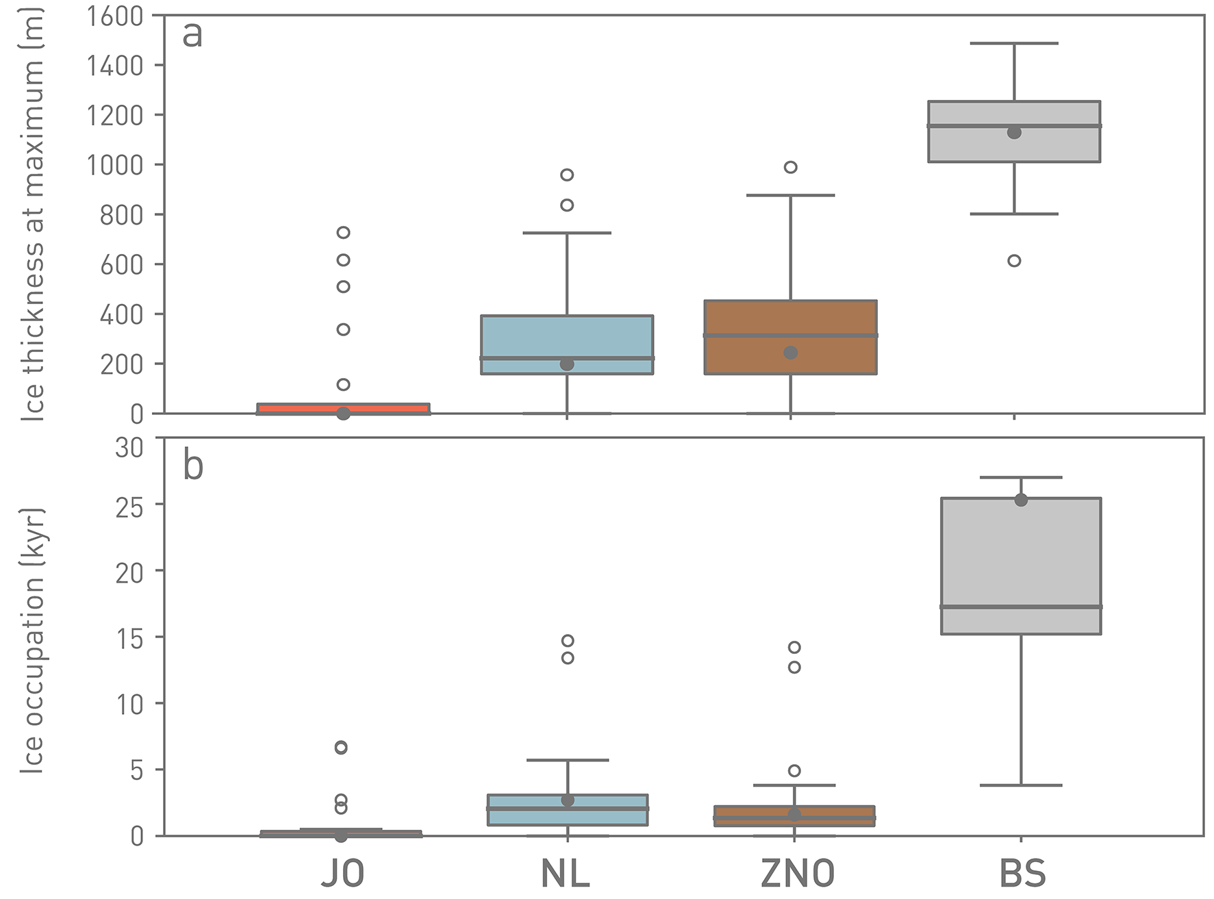
Fig. 6‑15:Boxplots of modelled ice characteristics during the LGM
(a) Maximum ice thickness and (b) Duration of ice occupation. The boxes depict data between the first (25th percentile) and third quartile (75th percentile) known as the interquartile range (IQR), while the grey line in the box shows the median value (50th percentile). Black solid points indicate the result from the reference simulation. From above the upper quartile, a distance of 1.5 times the IQR is measured out and a whisker is drawn up to the largest point from the dataset that falls within this distance. Similarly, a distance of 1.5 times the IQR is measured out below the lower quartile and a whisker is drawn up to the lowest point from the dataset that falls within this distance. All other points are plotted as outliers. Data are based on 19 simulations. See Fig. 6‑14 for the locations where ice thickness and duration of ice occupation were evaluated in the Jura Ost (JO), Nördlich Lägern (NL) and Zürich Nordost (ZNO) siting regions as well as for the Bodensee (BS) region.
These results are important for a variety of reasons. Firstly, they provide the boundary conditions for ice dynamics with respect to erosion potential. Secondly, ice loading affects mantle processes (e.g. Wu & Peltier 1982), which in turn cause transient perturbations of the stress field, including effects on uplift pattern and magnitudes (see Section 6.4 and Nagra 2024k) and may influence fault behaviour (see Section 6.2 and Nagra 2024l) and hydrogeological changes (Section 6.5). Assuming an ice density of 917 kg/m3 and mantle density of 3'300 kg/m3, a 400 m ice thickness could produce a lithospheric depression of up to ~ 110 m, if equilibrium is reached. Reaching equilibrium depends, in turn, upon the duration of the ice occupation and the viscoelastic response time influenced by the viscosity of the mantle. These parameters also influence the duration and magnitude of postglacial adjustment. Lithospheric glacial loading and unloading is accompanied by changes in vertical stress (sv) below the load but deviating horizontal stresses which extend beyond the ice cover (Grollimund et al. 2001, Steffen et al. 2022, Craig et al. 2023).
Basal ice temperature and sliding speed are two key variables that describe basal conditions relevant for glacial erosion (Fig. 6‑16). Glacial erosion occurs where ice is warm-based (not frozen to the ground), which enables basal sliding and thus abrasion. Furthermore, where meltwater is able to flow along the bed, this promotes rapid sliding and stimulates quarrying (plucking) or may directly lead to subglacial meltwater erosion. Simulations for the LGM indicate that basal ice reached the pressure melting point over much of the piedmont lobes of the Rhine Glacier system, and also in the glacial valleys that fed these lobes (Fig. 6‑16a). In the lobes, despite low surface slopes and low basal shear stresses in the Alpine Foreland, sliding dictated the main fluxes of ice, which closely followed bedrock topography. Ice was channelled between bedrock highs along troughs, some of which coincided with glacially eroded overdeepenings (Fig. 6‑16b). These sliding conditions favoured glacial erosion by abrasion and quarrying.
Assuming that the glacial erosion rate scales with the basal sliding speed, the sliding distance calculated by time-integrating the sliding speed (Näslund et al. 2003, Staiger et al. 2005, Yanites & Ehlers 2016) yields a metric for glacial erosion by moving ice. Transient ice-flow modelling of the Rhine Glacier system over the course of the last glacial cycle indicates that the sliding distance is greatest at the base of Alpine valleys where sliding is fastest and where ice occupation time is longest (Fig. 6‑16c). However, the sliding distance does not correlate well with the location of existing overdeepened valleys in the Alpine Foreland (Fig. 6‑16c) owing to the smaller sliding speeds near the ice margin and the short time period during which ice covered the distal foreland (Fischer et al. 2021).
Based on computed time-dependent ice surface elevations, maps of hydraulic potential and associated flow accumulation area are calculated to estimate the location of subglacial water drainage routes and water fluxes (Chu et al. 2016). Time-integration of the flow accumulation area yields a metric for erosion by subglacial water flow. Larger values of time-integrated flow accumulation area indicate zones with significant subglacial water flow that has the potential to enhance sediment removal and increase subglacial fluvial erosion. Results from simulations of the Rhine Glacier system during advance and retreat in the foreland indicate that subglacial water discharge was high and focused along glacial valleys and existing overdeepenings (Fig. 6‑16Fig. 6‑30d), in particular when the water pressure underneath the Rhine and Linth Glacier lobes was close to the ice overburden pressure. These conditions are necessary for subglacial water to remove basal sediments, expose fresh bedrock, and favour further glacial erosion. Knowledge of the location and fluxes of subglacial water drainage is therefore useful for understanding patterns of erosion beneath ice masses that do not otherwise relate to the sliding of ice (Cohen et al. 2023).
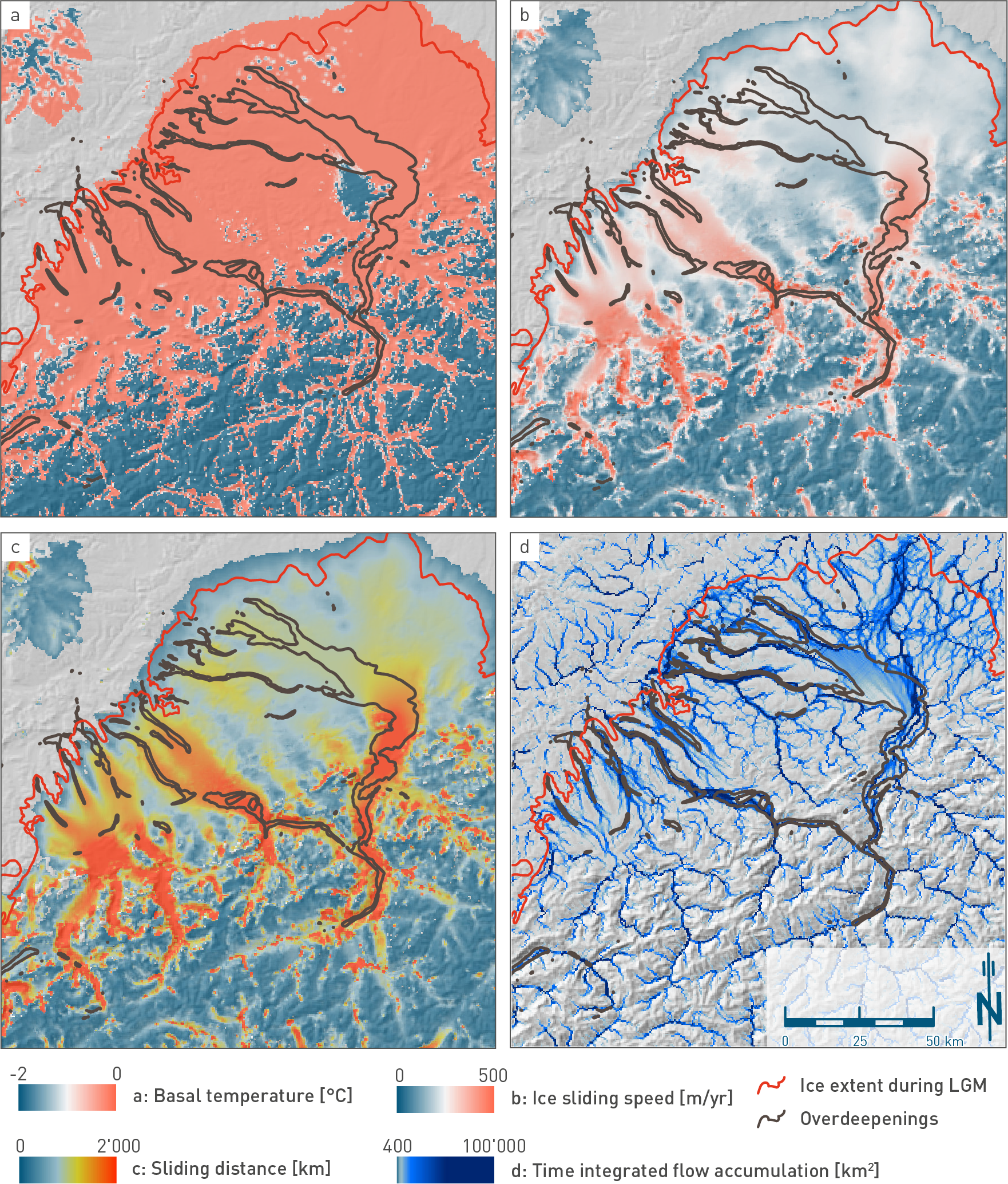
Fig. 6‑16:The Rhine Glacier system and erosion potential at the LGM
(a) Basal ice temperature. (b) Ice sliding speed. (c) Sliding distance calculated by integrating the sliding speed over the course of the last glacial cycle as a proxy for glacial erosion by moving ice. (d) Time-integrated flow accumulation area over 12.8 kyr around the LGM as a proxy for glacial erosion by subglacial water flow (see Nagra 2024j for more details). See Fig. 6‑14 for location. The brown lines denote the outlines of existing overdeepenings. The LGM extent is modified after Ehlers et al. (2011) and is shown by the red lines.