8. Analysis of radiological consequences (NTB 24-10)

The analysis of radiological consequences assesses the potential impact that radionuclide releases from the repository to the surface environment could have on a representative individual from the population group most affected living in the far future. The analysis demonstrates that the quantitative protection criteria in the form of maximum individual effective dose or risk as specified in the ENSI Guideline G03 (Section 2.4) are adhered to. It furthermore illustrates the system behaviour with respect to radionuclide release, retention and transport and shows ample safety margins.

While annual individual effective dose is the most relevant measure and is evaluated and compared with the regulatory dose criteria for all calculation cases, the risk criterion is (solely) applied for the “what-if?” case of “excavation of the repository by erosive processes” during the time period for assessment.

In Section 8.1, we summarise the methodological aspect for the radiological consequence analysis and how it is embedded in the general safety assessment workflow. The main results are then presented for the safety scenarios and “what-if?” cases in Sections 8.2 to 8.5 and an overarching summary is given in Section 8.6.

Note that the full details of the radiological consequence analysis are, in general, documented in Chapter 7 of NTB 24-18 (Nagra 2024p); for the calculations linked to future human action scenarios see Chapter 4 of NAB 24-09 (Nagra 2024r) and for the “what-if?” case of an “excavation of the repository by erosive processes” see Chapters 3 and 4 of NAB 24-08 Rev. 1 (Nagra 2024q). Furthermore, the computation results are digitally available as an electronic input data and results application (EDR, Nagra 2024p).

The embedding of the analysis of radiological consequences in the general safety assessment workflow (see Chapter 4 and Section 5.4 in NTB 24-19,Nagra 2024t) is illustrated in Fig. ‎8‑1. The starting point for the radiological consequence analysis is the set of calculation cases that has been defined in the safety scenario development as requiring quantitative evaluation, as discussed and illustrated in Chapter 7.

Each calculation case is then conceptualised in more detail. Numerical models are developed and parametrised, resulting in a set of calculations to be performed with input parameters for each of them. Care is taken that model abstractions are consistent with those made in PA and that related model uncertainty is bound and understood (see e.g., NAB 24-25, Nagra 2024k and Appendix A and E of NTB 24-18, Nagra 2024p).

The numerical models are composed of near- and far-field components to compute radionuclide release, retention and transport through the engineered barriers and the geosphere (i.e., the Opalinus Clay and the CRZ) and a biosphere model that converts release rates from the geosphere to the biosphere into annual effective doses (Fig. ‎8‑2).

In the near field, the focus is on the release (e.g., degradation and release rates, solubility) and retention (e.g., sorption) of radionuclides. The radionuclide source term is based on the expected inventory as described in Section 5.3.1. Due to the excellent retention properties of the repository barrier system, particularly the CRZ, only a small fraction of the radionuclides needs to be considered when calculating dose rates. These are determined using a screening process, which is based on a highly conservative and simplified transport model and, for the probabilistic calculations, in a second step based on the results of the deterministic calculations. Refer to Section 5.4.1. in NTB 24-19 (Nagra 2024t) for details.

For radiological consequence analysis, the stratigraphic units (host rock and confining units) are considered based on the abstraction shown in Fig. 7‑2 in Section 7.2.2. The geological units are considered as individual transport media in the numerical modelling, whereby some further abstractions are made, such as merging Calcareous Lias CL and Argillaceous Keuper AK3 to a unit KEU. The Keuper aquifer is part of the KAL unit in the numerical abstractions.

For the migration of radionuclides to the boundary of the CRZ, two pathways are considered:

• radionuclide migration in the aqueous phase, in which radionuclides are released to porewater that contacts the waste packages and are subsequently transported by aqueous diffusion and, where there is porewater flow, by advection, and

• radionuclide migration of ¹⁴C in both the liquid and gaseous phase¹⁸, in which ¹⁴C in the form of methane mixes with, and is transported by, other repository-generated gas (hydrogen).

The near-field and geosphere conceptualisations and models for the two pathways differ as follows¹⁹:

• For the aqueous phase calculations, the near field includes either an individual SF or RP-HLW disposal canister, together with its surrounding bentonite buffer, or an individual L/ILW emplacement cavern. The HLW and its surrounding near-field barriers are represented using radially symmetric geometries, while a 2D symmetric representation of the LK90 disposal cavern as described in NAB 23‑01 (Nagra 2023a) is used for the L/ILW near field. The near-field radionuclide release rates from SF and from RP-HLW are computed using the STMAN code (Robinson 2022). Releases from L/ILW are computed with the VPAC code. The main model output providing a source term for geosphere modelling is the total (positive) radial radionuclide flux across the emplacement drift or cavern into the surrounding rock. The geosphere retention and transport model is imple­mented in the PICNIC-TD code (Robinson & Chittenden 2022). The geosphere is modelled as a network of one-dimensional transport paths (called legs), which may represent porous media or discrete features such as fractures, cracks, or channels. Flow and transport parameter values, such as diffusion coefficient, sorption coefficient, and hydraulic con­ductivity, are assigned to each leg and are assumed to be invariant in time and space within an individual leg. The radionuclide flux from different exfiltration points from the leg structure is captured and summed together to obtain the release rate from the geosphere into the biosphere. 

• For the two-phase flow calculations, a 3D model combining both the near field and the geosphere is used. The implementation is based on the TOUGH3 code with its equation-of-state EOS75R module²⁰. It simulates two-phase flow of a gas phase and an aqueous phase and advective- diffusive transport of ¹⁴C as methane, with fully implicit thermo-hydro-mechanical coupling between primary variables (i.e., the state variables of pressure, gas saturation, temperature, mass fractions) and secondary variables (porosity, fluid density, fluid viscosity, capillary pressure) (Jung et al. 2018, Zhang et al. in prep.). In order to account for the different needs of dimen­sionality and discretisation in the near field and geosphere, a so-called “macro-element” approach is adopted, by which the number of the numerical elements is significantly reduced by simplifying the similar and (quasi) symmetrically positioned repository structures along with the surrounding rock to representative macro-elements. ¹⁴C fluxes from the model boundary are captured and summed together to obtain the release rate from the geosphere into the biosphere.

The biosphere model serves to convert radionuclide fluxes to an effective dose by providing so-called biosphere dose conversion factors (BDCFs). These BDCFs are derived from modelling of radionuclide transfer and accumulation processes in the surface environment and of radionuclide pathways leading to the exposure of humans to radioactivity. The biosphere modelling is carried out using a compartment modelling framework and is implemented with the SwiBAC code. For details of the biosphere modelling approach, see NAB 24-06 (Nagra 2024n). The biosphere model is identical for most calculation cases (use of reference biosphere), albeit for the reference safety scenario four different biosphere situations are considered, leading to four separate calculation cases (reference calculation case and three additional calculation cases, as shown in Fig. ‎7‑3). Only the “what-if?” case “excavation of the repository by erosive processes” and some future human action safety scenarios require adaptations of the biosphere model due to potential radionuclide sources directly in the surface environment (for details see NAB 24-08, Nagra 2024q and NAB 24-09, Nagra 2024r).

Note that in general, conservatively, radionuclide fluxes out of the CRZ are directly multiplied by the BDCFs. This corresponds to neglecting the transport time in between the boundary of the CRZ and the biosphere near-surface aquifer, that is, not taking credit for radioactive decay or for dispersion and dilution during this transport. This is illustrated in the scenario figures with the blue dashed lines (e.g., Fig. ‎7‑3).

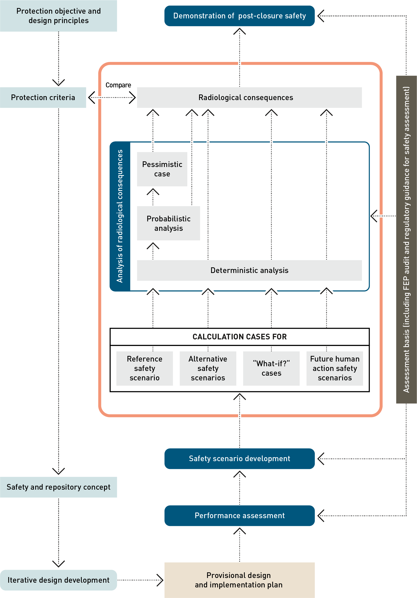
Fig. ‎8‑1:Workflow for the post-closure safety case, highlighting, in the orange box, the main elements of the analysis of radiological consequences

When parametrising the models used in calculations, care is taken to distinguish between realistic (best estimate) values, conservative or pessimistic assumptions, and stylised approaches (see also Section 4.4). In general, when there is quantified uncertainty in the properties of repository features, rates of processes and other model parameters, realistic values and, for the probabilistic calculation case, realistic parameter bandwidths, are assumed. Other uncertainties are generally handled using conservative assumptions. Parameter assumptions and details of the treatment of parameter uncertainty can be found in Appendix C in NTB 24-18 (Nagra 2024p). Stylised assumptions are made where appropriate. They are used in the context of the biosphere modelling, the “what-if?” case of “excavation of the repository by erosive processes” and future human actions safety scenarios. Further, the assumption is made that the different biospheres (e.g., constant climatic conditions) are maintained throughout the time period for assessment.

Once the models and parametrisations are defined, simulations are performed and the results are grouped in the electronic input data and results application (EDR, Nagra 2024p) such that each result can be linked to its input parameters and model chain. Finally, the results are compared with the regulatory protection criteria and the safety margins are evaluated. For this, dose rates as a function of time and the maximum dose rate over the time period for assessment are analysed and compared. For the calculation cases linked to the “what-if?” case of “excavation of the repository by erosive processes”, the risk is also evaluated and compared with the regulatory risk criterion for these calculation cases.

Organic ¹⁴C is considered as methane in both the aqueous phase calculations and in the two-phase flow calculations. Because the entire organic ¹⁴C inventory is considered separately in both calculations, the results are also presented separately as alternative model assumptions, i.e., one in which all methane is assumed to be fully dissolved despite its volatility and the low solubility of methane gas and one in which methane is partitioned between the dissolved and gaseous phases. In fact, summing both results would correspond to counting the organic ¹⁴C inventory twice. A further reason for presenting the results separately is that otherwise the distinct characteristics of the two-phase flow results would be barely visible, since the absolute values of dose rate contributions for these cases are small when compared with the aqueous phase contributions.

Note that, in the graphical representation of the radiological dose calculations shown in the following sections, the grey-shaded areas indicate two aspects:

• Dose rate: Many of the calculations presented in this chapter show very low dose rates. A dose of 10^-7 mSv/a to an individual corresponds to an extremely low overall fatal risk coefficient for the exposed person of 5 × 10^-12 per year²¹. This is reflected in the graphical presentation of such results, where grey shading is used below 10^-7 mSv/a to emphasise that such results have no radiological significance.

• Extended time period: Shading is also used in graphs of dose-rate evolution, where results are presented beyond the time period for assessment of one million years, again to illustrate the behaviour of the models representing the disposal system, as well as to ensure that maximum dose rates are captured.

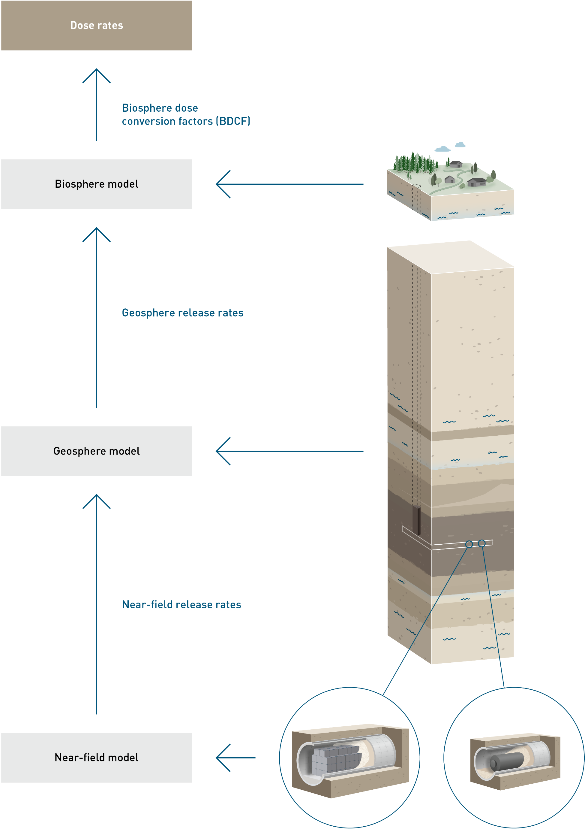
Fig. ‎8‑2:Workflow for the computation of radiological consequences for an individual calculation

The reference safety scenario represents the expected initial state and expected evolution over time. Several deterministic calculation cases and one probabilistic calculation case, as summa­rised in Tab. ‎8‑1 and described in Section 7.2, have been defined for the reference safety scenario. Calculation cases for the reference conceptualisation of the CRZ cover the reference case, alternative climatic conditions and one different geomorphology (different biospheres), and one calculation case addresses parameter uncertainty. An additional calculation case uses a variant conceptualisation of the CRZ with a hydraulically inactive Keuper aquifer to account for uncertainty in geological characterisation.

Computed dose rates for the reference calculation case RS-RC resulting from radionuclide migration in the aqueous phase are shown in Fig. ‎8‑3, where the contributions of the HLW (top), L/ILW (middle) and the total dose rate for the repository (bottom) are distinguished. In each subfigure, the radionuclides that contribute significantly (and visibly) to the total dose rate are also plotted. It becomes obvious that only three radionuclides, namely I-129, Cl-36 and Se-79, reach the biosphere in sufficient amounts to contribute to the dose rates. Ca-41 only appears in the dose rate in which the contributions from both HLW and L/ILW are combined and has no radiological significance. All the other radionuclides decay to such a degree during their transport from the waste through the near field and the CRZ that their contributions are negligible, i.e., below 10^‑9 mSv/a, and thus not visible in the plots. The three contributing types of radionuclides are characterised by a sufficiently large inventory, low sorption coefficients, and comparably long half-lives.

While the relative contribution of the three radionuclide types differs between the L/ILW and HLW repository sections, and also changes over time, it is clearly the HLW repository section that dominates the overall dose rates, with I-129 being the radionuclide with the highest contribution.

The total dose rate reaches 1.5 × 10^-4 mSv/a after one million years, which is about three orders of magnitude lower than the protection criterion of 0.1 mSv/a, indicating a large safety margin. Note that the total dose rate continues to increase slightly thereafter, reaching a maximum of 2.0 × 10^-4 mSv/a after about 4.5 million years, but remains about four orders of magnitude below the typical present-day natural radiological exposures in Switzerland and as published by the Swiss Federal Office of Public Health in their annual reports on radiological monitoring of the environment (“Umweltradioaktivität” BAG 2021). 

A more detailed analysis of the radionuclide transport distance while considering decay is provided by analysing the dose rate contribution of radionuclides as a function of the distance from the near field (Fig. 8‑4). For this, selected radionuclide fluxes were captured in the geosphere model every 10 m, and a hypothetical dose rate contribution per radionuclide was computed, assuming that the exfiltration pathway would be at these locations, i.e., the radionuclide fluxes at these hypothetical interfaces every 10 m were converted to dose rates using the BDCF from the reference calculation case. The excellent retention capacity of the near field as well as that of the Opalinus Clay (OPA) become evident. The same radionuclides as in Fig. ‎8‑3 (I-129, Cl-36, Se-79 and Ca-41) leave the host rock and penetrate further into the upper (UCU) and lower confining geological units (LCU) and eventually reach the biosphere.

Tab. ‎8‑1:Calculation cases for the reference safety scenario

All cases are calculated using both modelling approaches: aqueous-phase transport and two-phase transport of ¹⁴C.

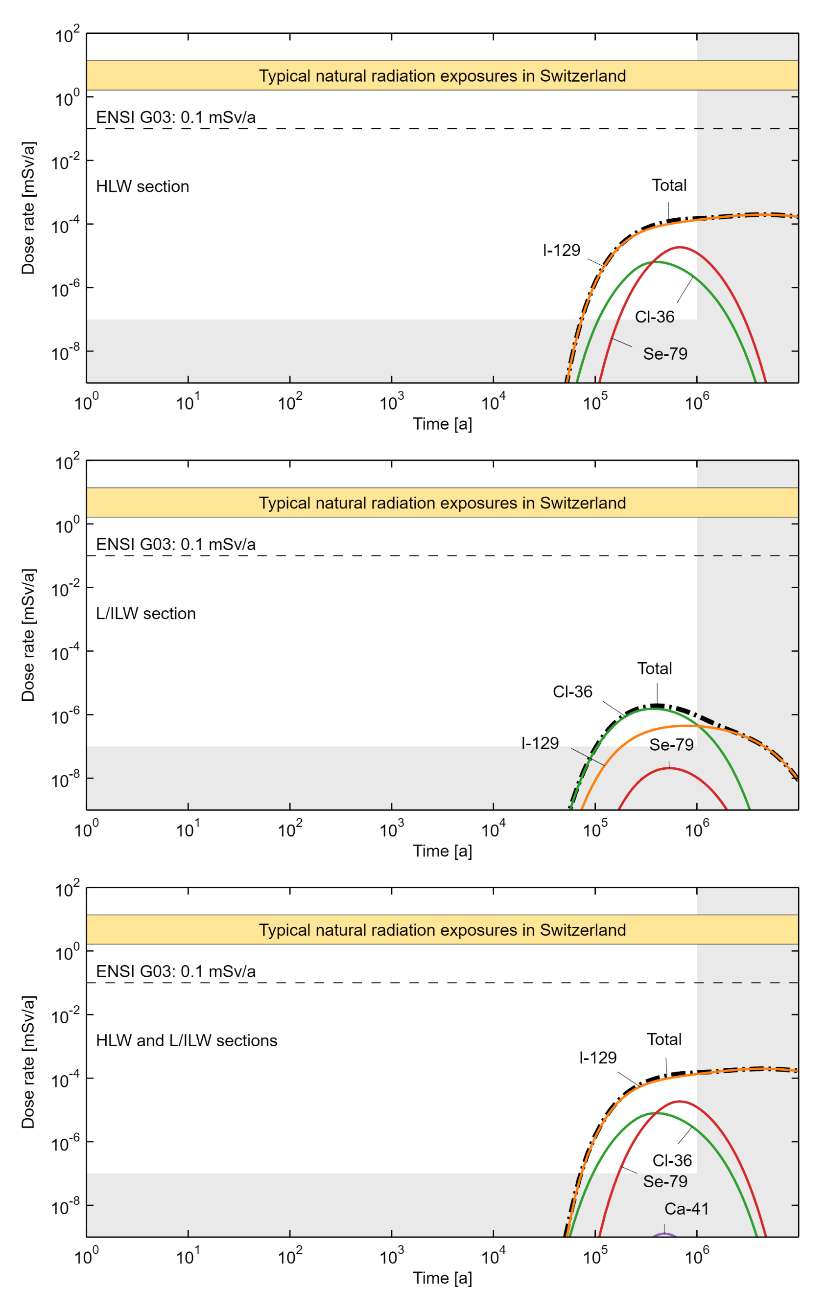
Fig. ‎8‑3:Dose rates and main contributing radionuclides for the reference calculation case RS-RC assuming radionuclide transport in the aqueous phase

Contribution from HLW repository section (top); contribution from L/ILW repository section (middle); total dose rate for the repository (bottom).

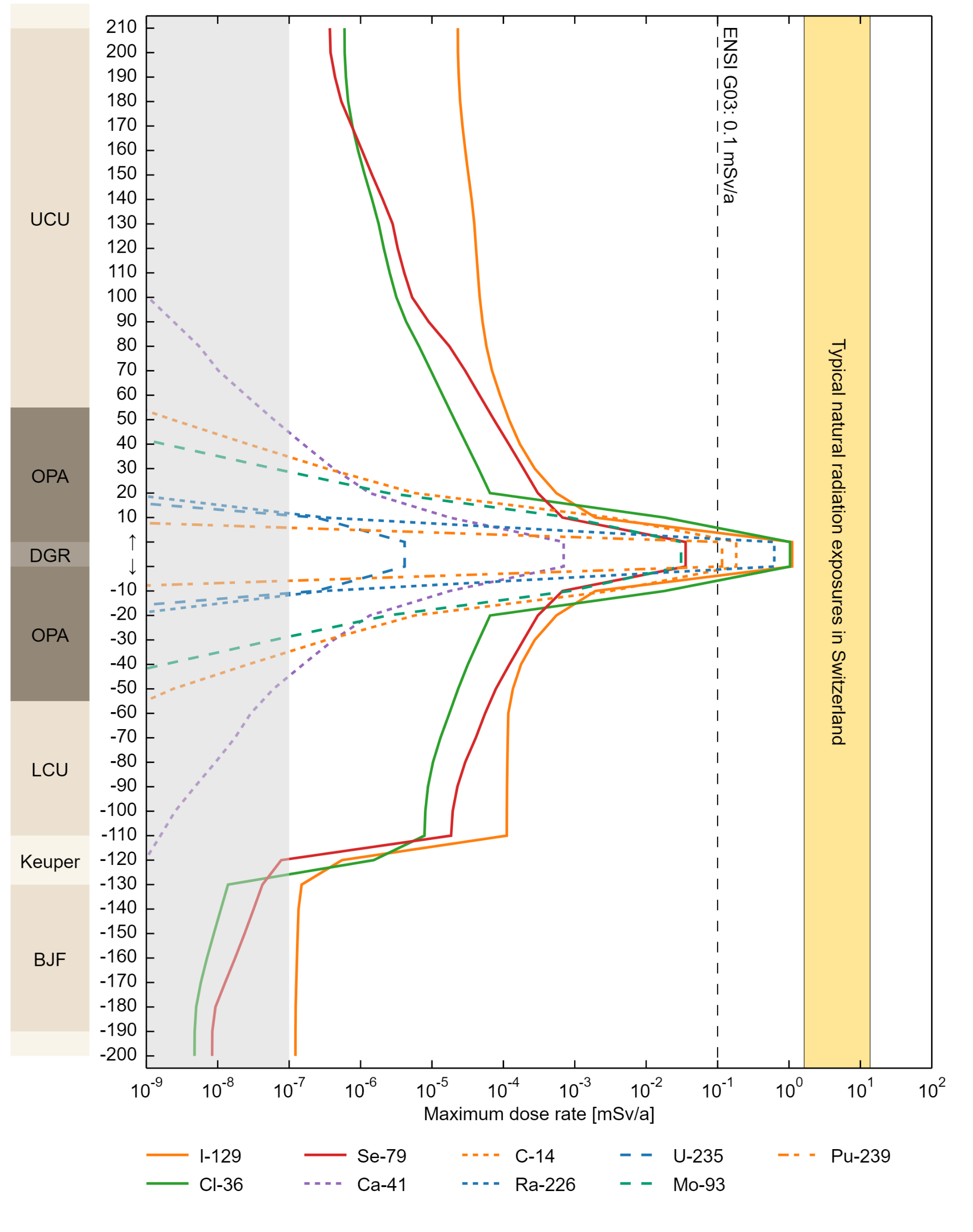
Fig. ‎8‑4:Hypothetical dose rate contributions of individual radionuclide types for the refer­ence calculation case RS-RC in the aqueous phase based on radionuclide fluxes captured in the near field (one value) and every 10 m in the geosphere model

UCU = upper confining geological units, OPA = Opalinus Clay, DGR = deep geological repository, LCU= lower confining geological units, BJF = Bänkerjoch Formation, groundwater markers indicate the deep groundwater aquifers: Malm (at the top of the UCU), Keuper (in-between the LCU and the BJF) and Muschelkalk (below the BJF). For a selected dose rate on the x-axis (e.g., 10^‑5 mSv/a), the reading of the distance on the y-axis (e.g., -30 m) indicates how far a signal of a given radionuclide, expressed as maximum dose rate contribution, reaches (e.g., Ca-41 would contribute ca. 10^‑6 mSv/a if the flux of Ca-41 at 30 m into the geosphere could be captured and directly transferred into the biosphere aquifer). Radionuclides with dashed lines would contribute less than 10^‑7 mSv/a at the boundary of the Opalinus Clay, ca. 50 m away from the centre of the repository into the geosphere. The sharp drop in the Keuper is due to dilution effects in the aquifer.

One key result of the probabilistic calculation case for the reference safety scenario, RS-PROB, is shown in Fig. ‎8‑5. The bandwidth of calculated dose rates assuming radionuclide transport in the aqueous phase is shown using the statistical measures of median, 95/5 and 84/16 percentiles, and the maximum and minimum dose rates (individually computed at each time step as maximum and minimum across all the probabilistic calculations).

The dose rates for the probabilistic calculation case remain comfortably two orders of magnitude below the dose protection criterion of 0.1 mSv/a, thus demonstrating an ample safety margin with respect to parameter uncertainty.

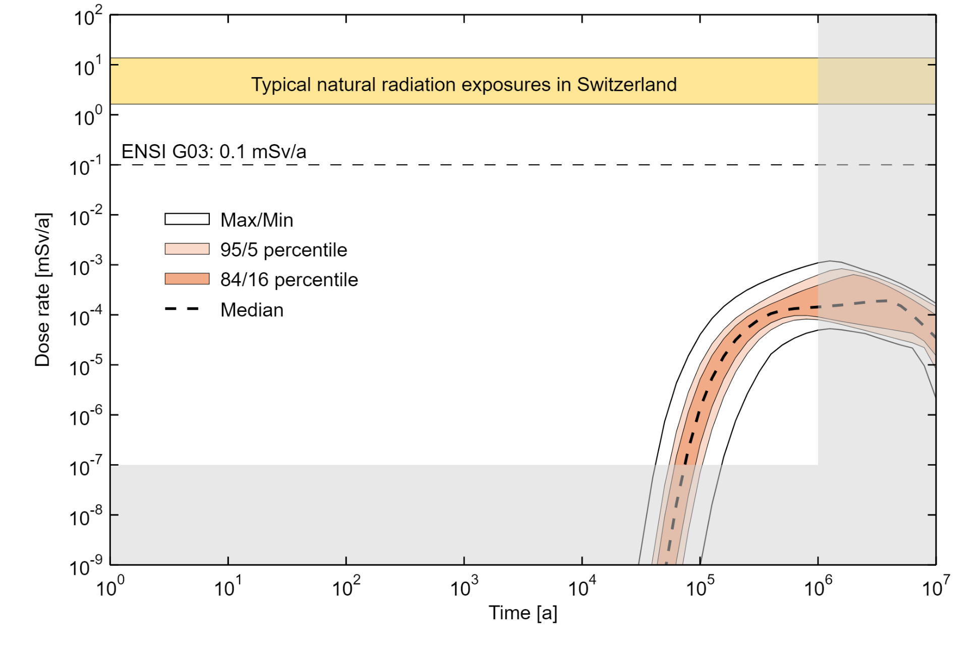
Fig. ‎8‑5:Dose curves and bandwidths for the probabilistic calculation case assuming radionuclide transport in the aqueous phase

The statistical measures of median, 95/5 and 84/16 percentiles, and the maximum and minimum dose rates individually computed each time as maximum and minimum across all the probabilistic calculations are shown (i.e., the Max/Min lines do not correspond to one calculation case).

So far, we have summarised the results of the reference calculation case and the probabilistic calculation case for the reference safety scenario when considering radionuclide transport in the aqueous phase only. In fact, this is the pathway that contributes most to the dose rates and dominates them. This is illustrated in Fig. ‎8‑6 which shows the maximum dose rates calculated for the probabilistic calculation case RC-PROB in the form of two boxplots, one where only aqueous phase transport is modelled for all the radionuclides (left side) and one for ¹⁴C which, in the form of methane, is the only radionuclide that could significantly contribute to dose rates by migration in the gaseous phase (right side). The maximum dose rates are orders of magnitude smaller in the latter case.

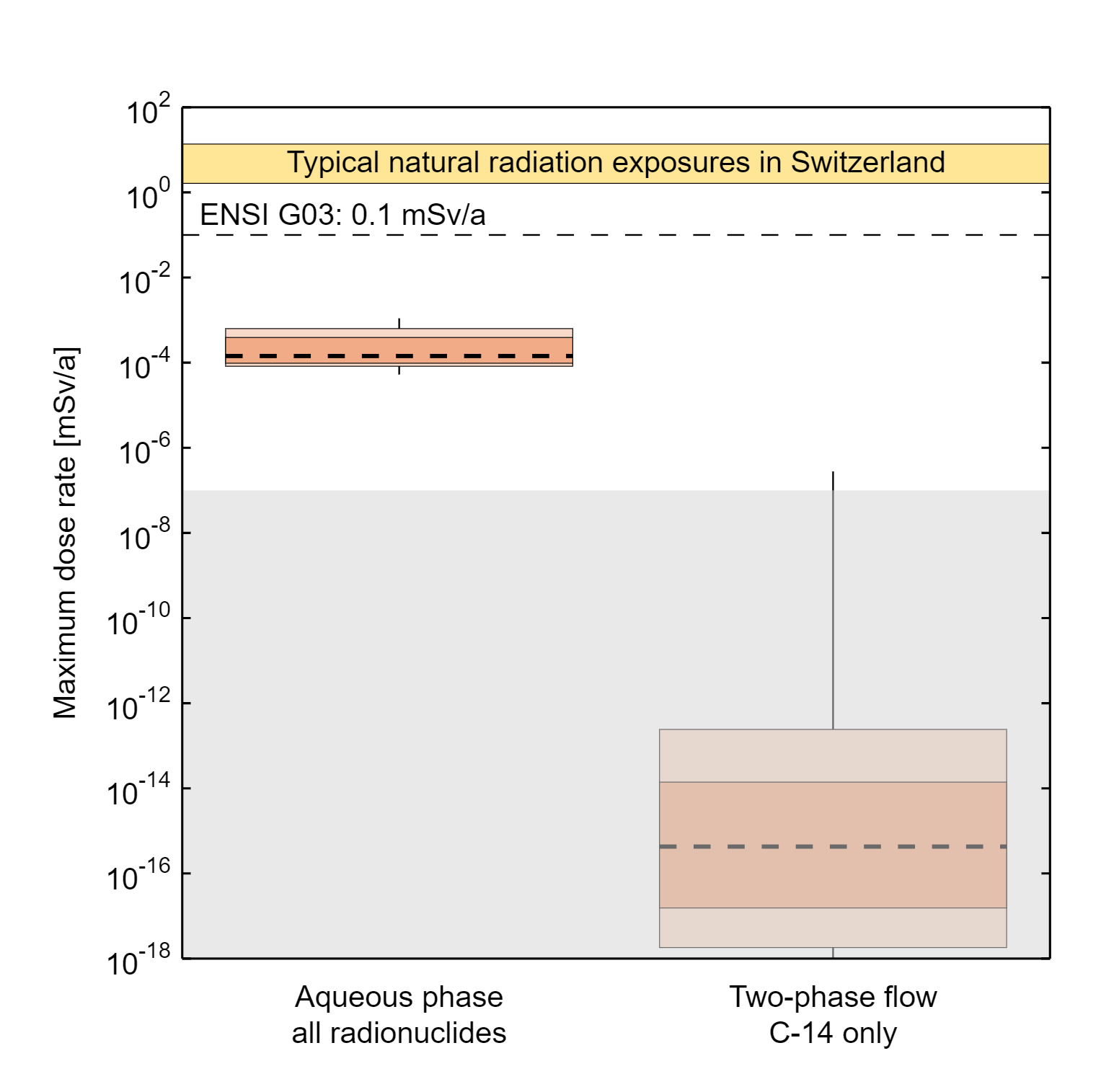
Fig. ‎8‑6:Summary showing the maximum dose rates for the probabilistic calculation case for the aqueous phase transport (left) and two-phase transport of ¹⁴C (right)

The maxima are calculated over a total calculation period of 10⁶ years (see Fig. ‎8‑5). The boxplots show the statistical measures of median (dashed horizontal line), 95/5 and 84/16 percentiles (light and dark shades of red) and the full extent of the spread between minimum and maximum (thin vertical line).

Both the ample safety margin and the dominance of the aqueous phase transport path are confirmed when analysing the dose rates for all the deterministic cases linked to the reference scenario (Fig. ‎8‑7). For the aqueous phase transport (Fig. ‎8‑7a), the results for the warmer and drier biosphere (RS-BIOS/WARM_DRY) and for the pessimistic calculation case (RS-CMB) lead to dose rates that are roughly within the probabilistic bandwidth of the calculation case RS-PROB. However, they are – expectedly – higher than the dose rates of the reference calculation case (RS-RC). The results of the calculation case with assumptions of the inactive Keuper aquifer below the HLW repository section (RS-KEUPER_INACTIVE) and of the two cases with a colder (RS-BIOS/COLD) or a drained farmland biosphere (RS-BIOS/DRAINED_FARMLAND) with lower BDCFs, lead to dose rates that are one to four orders of magnitude below those of the reference calculation case – leaving very large safety margins.

In Fig. ‎8‑7b, the dose rate for the pessimistic calculation case RS-CMB is shown for the two-phase transport of ¹⁴C (mainly transported as methane). It is larger than 10^-7 mSv/a for a short time – but still very low. The resulting dose rates for the other deterministic calculation cases for the reference scenario and this transport pathway all remain below 10^-9 mSv/a.

Fig. ‎8‑7:Dose curves for the reference case and for other deterministic calculation cases with­in the reference scenario, showing the contributions of aqueous phase transport (a) and two-phase transport of ¹⁴C (b)

In summary, both the probabilistic and deterministic results for the reference safety scenario demonstrate that the regulatory dose protection criterion is respected. The probabilistic results show a safety margin of more than two orders of magnitude for the 95 percentile and close to three orders of magnitude for the median. The most pessimistic deterministic case has a maximum dose rate occurring after roughly one million years that is still about two orders of magnitude below the regulatory protection criterion. Thus, for the expected evolution of the repository and considering parameter uncertainty within this evolution path, it can be demonstrated with a high level of confidence that humans and the natural environment will not be exposed to harm.

As described in Section 7.3, two alternative safety scenarios that address uncertainties in geological characterisation have been identified:

• one of the confining geological units above (variant one) or below the Opalinus Clay (variant two) provides a horizontally connected advective pathway connected to the regional aquifer, and thus provides an additional pathway for advective transport of radionuclides,

• an undetected fault, with a transmissivity that is in the range of what could reasonably be expected in such a scenario, exists in the vicinity of the repository at the time of its construction. The undetected fault could intersect either the HLW or the L/ILW repository section, leading also to two variants for this alternative safety scenario.

Finally, sets of calculation cases are considered for the two alternative safety scenarios as summarised in Tab. 8‑2 and Tab. 8‑3 (for details and illustrations see Section 7.3). Tab. 8‑2 also indicates which radionuclide transport pathways are considered for which calculation case for the first alternative scenario. In fact, since gas-phase-mediated transport is directed upwards, the two-phase flow computation accounting for ¹⁴C as methane is used -conservatively- for the closest hydraulically active unit above the repository.

Tab. ‎8‑2:Calculation cases for the alternative safety scenario that assumes an additional hydraulically active unit within the CRZ above or below the Opalinus Clay

The transport modelling approach refers to the two modelling approaches: one that assumes all radionuclides dissolve and migrate through the repository barrier system in the aqueous phase, and one in which gaseous ¹⁴C migrates, along with other repository-generated gas, in a two-phase flow regime. Only case AS-HA/SCD is modelled by the latter approach, since this is the most conservative case.

Tab. ‎8‑3:Calculation cases for the alternative safety scenario that assumes an undetected fault.

All cases are calculated using both modelling approaches: aqueous-phase transport and two-phase transport of 14C.

The results in the form of dose rates are shown for all the calculation cases of the alternative safety scenarios in Fig. 8‑8 for both (a) the aqueous phase and (b) two-phase transport. For the aqueous phase results, the reference case is also shown for comparison (for two-phase transport, the dose rate for the reference case is negligible). It can be easily noted that the presence of hydraulically active units has a limited effect on the results. Dose rates can increase minimally, and appear only slightly earlier compared with the reference case.

In contrast, the presence of an undetected fault could lead to releases to the biosphere at significantly earlier times, especially in the cases when the fault intersects the L/ILW emplace­ment caverns. An undetected fault also leads to a noticeable – albeit still very low – dose rate contribution of ¹⁴C as methane that migrates via a gas phase. However, for this alternative safety scenario, the overall dose rate maxima are again only marginally affected.

In general, similarly comfortable safety margins remain when compared with the reference safety scenario.

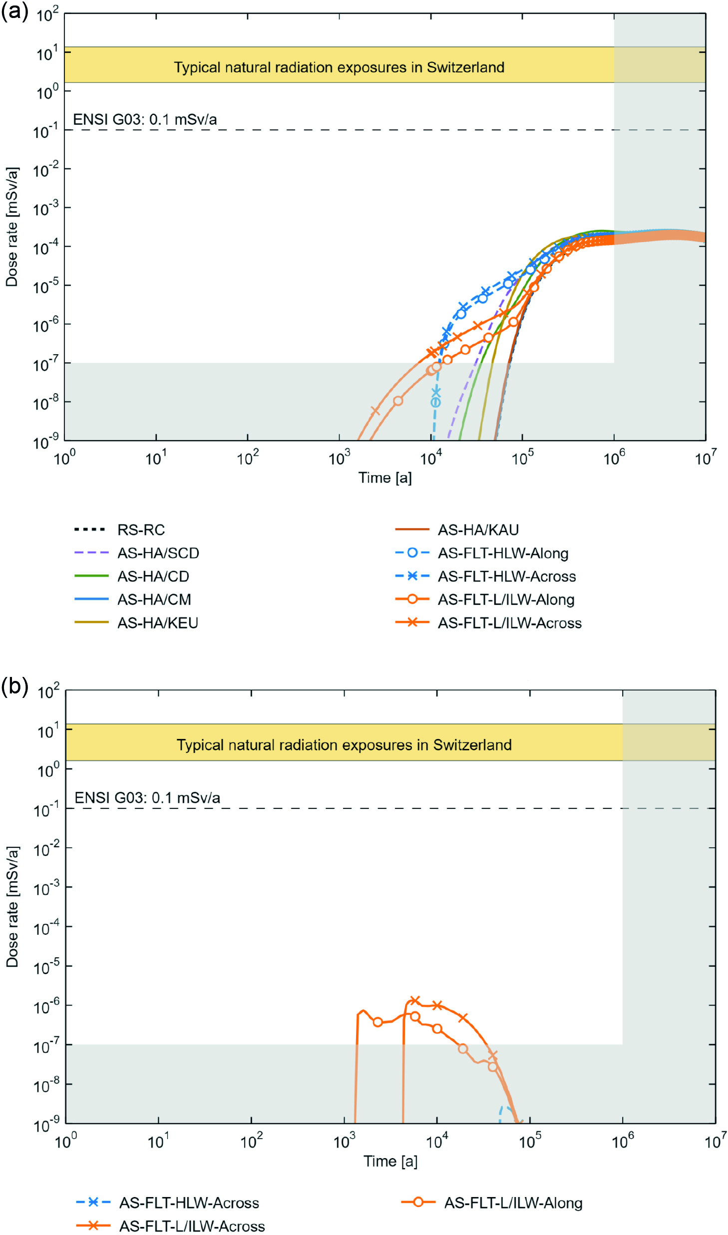
Fig. ‎8‑8:Dose curves for the calculation cases of the alternative safety scenarios and radionuclide transport in (a) the aqueous phase and (b) for the two-phase transport of ¹⁴C (only 3 cases lead to dose rates higher than 10^-9 mSv/a)

As discussed in Section 7.4, “what-if?” cases are split into those related to real physical phenomena and additional hypothetical cases with degraded or removed pillars of safety.

Occurrence of an undetected fault with a hypothetically high transmissivity in the vicinity of the repository

Two “what-if?” cases related to the physical phenomenon of geological faults were identified (see Section 7.4.1):

• the occurrence of an undetected fault with a hypothetically high transmissivity in the vicinity of the repository,

• the future creation or re-activation of a fault either by geological processes or as a repository-induced effect after repository closure.

For each of these “what-if?” cases, two variants consider whether the HLW or L/ILW repository section is affected and two calculation cases per variant address the fault orientation. The calculation cases are summarised in Tab. 8‑4 and Tab. 8‑5. For details and illustrations see Section 7.4.1. Note that the different timing of fault re-activation for the HLW and L/ILW variants corresponds to conservative assumptions with respect to potential radiological consequences (see Section 7.4.1)

Tab. ‎8‑4:Calculation cases for the “what-if?” cases for an undetected fault with hypothetically high transmissivity

All cases are calculated using both modelling approaches: aqueous-phase transport and two-phase transport of ¹⁴C.

Tab. ‎8‑5:Calculation cases for the “what-if?” cases for fault re-activation by geological processes or as a repository-induced effect

All cases are calculated using both modelling approaches: aqueous-phase transport and two-phase transport of ¹⁴C.

The results in the form of dose rates are shown for the calculation cases of these “what-if?” cases in Fig. 8‑9 for both (a) the aqueous phase and (b) two-phase transport. For the aqueous phase results, the reference case is also shown for comparison (for two-phase transport, the dose rate for the reference case is negligible).

The two calculation cases with an undetected fault with hypothetically high transmissivity intersecting L/ILW emplacement caverns (WI-FLT-L/ILW-Along and -Across) have highest dose rates for the aqueous phase, being about one order of magnitude below the dose protection criterion (Fig. ‎8‑9a). There is not a big difference between the fault with strike running along the axis of a single emplacement cavern and the one striking perpendicular to caverns, cutting each cavern at its centre. The calculation cases of a newly created or re-activated fault after 20,000 years intersecting L/ILW emplacement caverns (WI-FLT/RA-L/ILW-Along and -Across) have much lower dose rates that are only one order of magnitude above the reference case.

The dose rates for similar calculation cases for faults intersecting the HLW emplacement drift(s) are more than one order of magnitude below the dose protection criterion. The calculation cases WI-FLT-HLW-Along and WI-FLT-HLW-Across are almost identical to the calculation cases WI-FLT/RA-HLW-Along and WI-FLT/RA-HLW-Across and therefore not visible in Fig. 8‑9.

For the two-phase flow results (Fig. 8‑9b), the highest dose rates come from the same calcu­lation cases as for the aqueous phase, which are also about one order of magnitude below the dose protection criterion. WI-FLT-L/ILW-Across gives higher dose rates than WI-FLT-L/ILW-Along because the fault cuts each drift at its centre and the gas is able to escape from each cavern along the fault.

The HLW calculation cases for the two-phase flow are two orders of magnitude and more below the protection criteria. WI-FLT-HLW-Along is not visible in the figure since it is almost identical to WI-FLT/RA-HLW-Along.

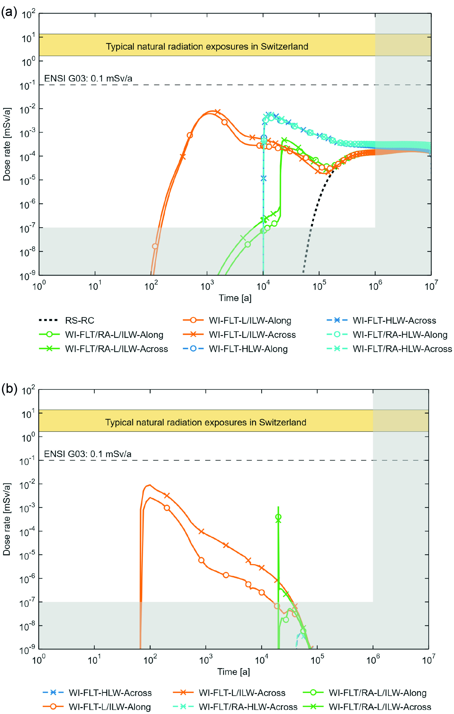
Fig. ‎8‑9:Dose rates for the calculation cases of the “what-if?” cases related to physical phenomena and radionuclide transport in the aqueous phase and (a) for the two-phase transport of ¹⁴C (b)

Excavation of the repository by erosive processes

An additional “what-if?” case related to physical phenomena concerns the excavation of the repository by erosion. During the time period for assessment, the occurrence of such an event has been demonstrated to be hypothetical (Nagra 2024i), thus positioning it as a “what-if?” case linked to the physical phenomenon of erosion. Note that, in the very distant future, beyond the one-million-year time period for assessment, there is a slow increase in probability with advancing time for repository material to be excavated as a result of erosion processes (NAB 24-08 Rev. 1, Nagra 2024q.

The variants and calculation cases for this “what-if?” case are shown in Tab. 8‑6 and Tab. 8‑7. The derivation of the variants and calculation cases, and also the radiological consequences of excavation of repository material by erosion, are fully discussed and analysed in NAB 24-08 Rev. 1 (Nagra 2024q). Uncertainties in key parameters, such as the assumed erosion rates, as well as the nature of the erosion (glacial and non-glacial), are taken into account and lead to the consideration of excavation occurring between 700,000 and four million years after repository closure.

Tab. ‎8‑6:Calculation cases for the assessment of repository excavation by deep glacial erosion

All calculation cases are calculated for excavation occurring 700,000 and 1, 2, and 4 million years after repository closure.

Tab. ‎8‑7:Calculation cases for the assessment of repository excavation by non-glacial erosion

All calculation cases are calculated for excavation occurring 700,000 and 1, 2, and 4 million years after repository closure.

To demonstrate regulatory compliance for times within the time period for assessment (see Sec­tion 2.4), the radiological consequences of repository excavation prior to one million years after repository closure are expressed in terms of annual risk and compared with the risk protection criterion of 10^-5 per year (Fig. 8‑10) because dose rates exceed 0.1 mS/year for some calculation cases (Sections 3.7 and 4.7 of NAB 24-08 Rev. 1, Nagra 2024q). The annual risk is more than two orders of magnitude below the risk protection criterion and is so low that any impact during this period can effectively be considered irrelevant.

For excavation times beyond the time period for assessment, i.e., beyond one million years, calculated dose rates are shown in Fig. 8‑11. The dose rates are below or within the range of natural radiation exposure in Switzerland, and therefore also compliant with the regulatory protection criterion for such long timescales (see Section 2.4).

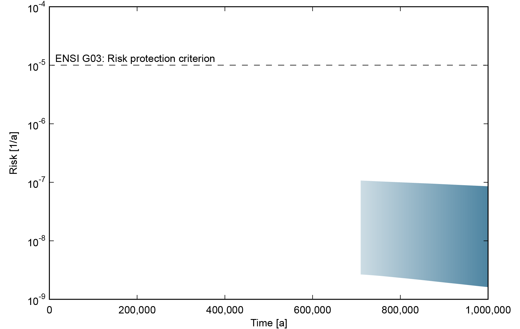
Fig. ‎8‑10:Illustration of the range of the annual risk associated with repository excavation compared with the regulatory risk protection criterion, for excavation times of up to one million years

Based on the calculated dose rates for repository excavation after 700,000 and 1 million years from NAB 24-08 Rev. 1 (Nagra 2024q), conservatively using the probability of excavation at one million years from (see Figure 6-44 of NTB 24-17, Nagra 2024i).

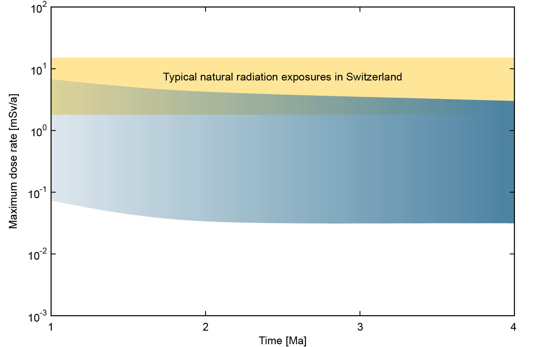
Fig. ‎8‑11:Illustration of the range of the maximum dose rates for excavation times after the time period for assessment (1 to 4 million years)

Based on the range of maximum calculated dose rates for all the calculation cases for the assessment of repository excavation by erosive processes after 1, 2 and 4 million years. The shading indicates an increase of probabilities of the excavation at later times.

Further “what-if?” cases are defined by systematically going through the pillars of safety and either removing them or assuming a degradation of the safety function they serve. The calculation cases as identified in the scenario development are summarised in Tab. 8‑8 (see Section ‎7.4 for details and illustrations). Tab. 8‑8 also indicates which radionuclide transport pathways are considered for which calculation case. On the one hand, calculation cases that impact mainly the flow along the underground structures, i.e., linked to the closure system or the permeability of the bentonite buffer, are only calculated for the two-phase flow and transport since the aqueous phase transport is dominated by diffusion through the CRZ. On the other hand, calculation cases that obviously do not significantly impact two-phase flow and release or the transport of ¹⁴C as methane are only computed for the aqueous phase. This concerns hypothetical assumptions of no sorption or solubility limits, hypothetically high dissolution rates for spent fuel or the glass matrix of reprocessed waste, and also hypothetically high diffusion coefficients in the bentonite buffer. Finally, the calculation case with a hypothetically high upwardly directed hydraulic gradient would lead to lower doses for the aqueous phase transport since the dominating transport path for radionuclides is downwards.

Tab. ‎8‑8:“What-if?” cases with hypothetically degraded performance of pillars of safety

The results in the form of dose rates for the “what-if`?” cases with hypothetically degraded pillars of safety are given in Fig. ‎8‑12 for both (a) the aqueous phase and (b) two-phase transport. For the aqueous phase results, the reference case is also shown for comparison (for two-phase transport, the dose rate for the reference case is negligible).

The aqueous phase results in Fig. ‎8‑12a show one calculation case with more than one order of magnitude higher maximum dose rates and considerably earlier releases than for the reference case; this is the calculation case of hypothetically high diffusion coefficients (WI-CRZ-DIFF).

Three calculation cases with hypothetically degraded performance of the CRZ lead to higher dose rates by up to about one order of magnitude and earlier releases than the reference case; this illus­trates the importance of the geological barrier. These three calculation cases are (i) no geosphere sorption (WI-CRZ-NOSORB), (ii) the upper and lower confining geological units are disregarded (WI-CRZ-NOCONFINING) and (iii) a hypothetically high downwardly directed hydraulic gradient (WI-CRZ-GRADdown).

Two additional calculation cases also show approximately one order of magnitude higher dose rates compared with the reference case: (i) hypothetically high instant release fractions (IRFs) for radionuclides in SF (WI-SF-IRF) and (ii) hypothetically high matrix dissolution rates for SF and RP-HLW (WI-HLW-DISS).

All the other calculation cases for the aqueous phase have no impact on the dose rates.

For the two-phase flow results (Fig. 8‑12b) only the dose rates from two calculation cases are visible; one with a hypothetically high diffusion coefficient for ¹⁴C (WI-CRZ-DIFF) and one with a hypothetically high permeability of the V3 seals (WI-V3). Only WI-V3 gives rise to dose rates above 10^-7 mSv/a.

Overall, the results of all the “what-if?” cases are well below the dose protection criterion, again confirming the robustness of the repository system.

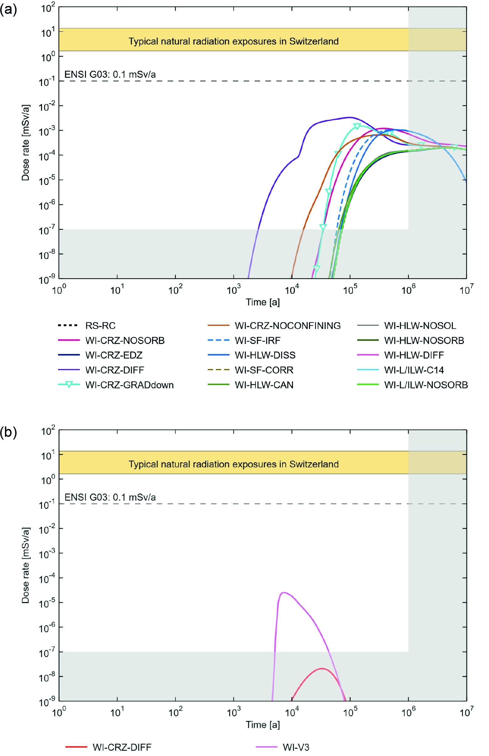
Fig. ‎8‑12: Dose rates for the calculation cases for the “what-if?” cases with hypothetically degraded performance of pillars of safety and radionuclide transport in the aqueous phase (a) and for the two-phase transport of ¹⁴C (b)

The following is a synthesis of the detailed results presented in NAB 24-09 (Nagra 2024r), where the derivation and the analysis of FHA safety scenarios are described in detail.

Two FHA safety scenarios have been identified for quantitative analysis (see Section 7.5):

• direct hit of the disposal canisters / containers by a deep borehole (FHA-1),

• abandonment of the repository (FHA-2).

For FHA-1, two variants with two or three calculation cases are propagated to radiological consequence analysis, while for FHA-2 only two calculation cases are propagated. A summary is provided in Tab. ‎8‑9 (for details, see Section 7.5). Note that, within a calculation case, different parametrisations were used to explore sensitivities and the impact of remaining uncertainties (see Chapter 3 of NAB 24-09, Nagra 2024r for details).

Tab. ‎8‑9:Calculation cases for the FHA safety scenarios

Within a calculation case, several parametrisations may be used to explore sensitivities and the impact of remaining uncertainties.

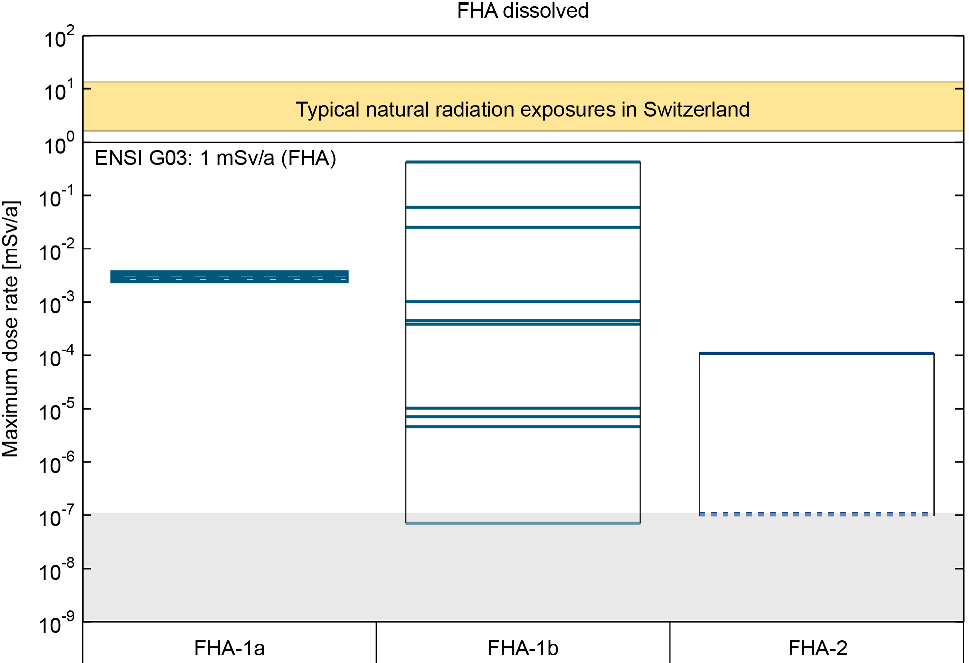
The results of the FHA dose calculations are summarised in Fig. ‎8‑13, which provides an overview of the maximum dose rates for the different calculations performed.

The spread of the results highlights the dependency of the radiological consequences on the details of a future borehole placement and penetration. In particular, the release of the rather short-lived ¹⁴C via a gaseous phase and the conservative assumptions of instantaneous and non-limited dissolution of the L/ILW inventory for the aqueous phase calculations lead to strong dependencies on assumptions such as, e.g., the penetration time or the flow regime along the borehole.

Nevertheless, and despite the conservative assumptions, the maximum dose rates for all the FHA calculation cases are considerably below the regulatory limit for FHA (i.e., 1 mSv/a).

 (a)

(b)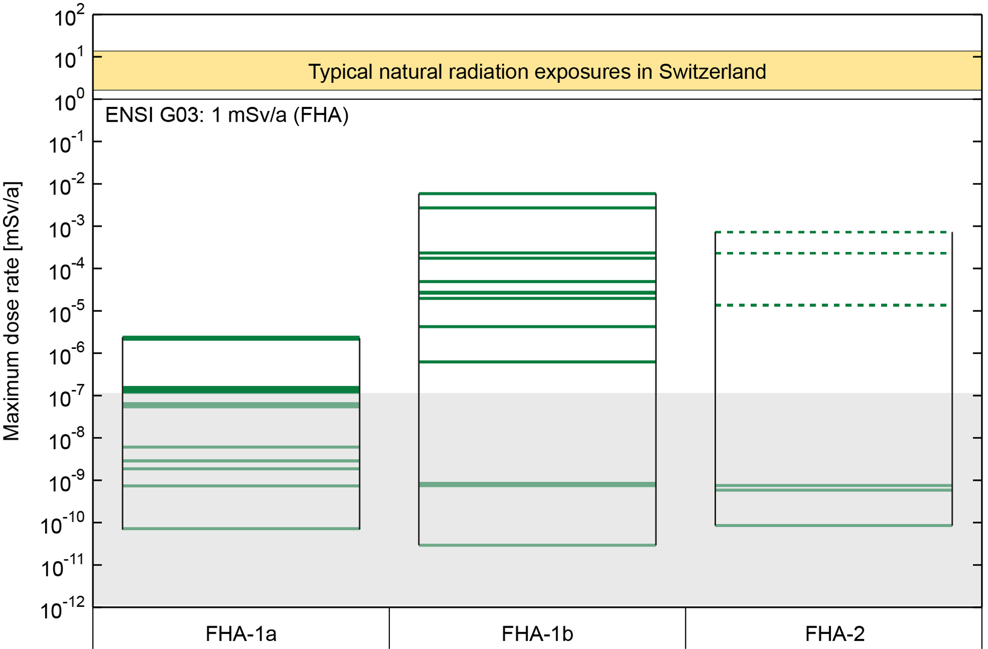

Fig. ‎8‑13Summary figure showing the maximum dose rates over 10⁶ years for the future human action calculation cases for the aqueous phase transport of all radionuclides (a) and for two-phase transport of ¹⁴C (b)

The spread of the results is due to the different calculation cases and, within the calculation cases, different parameterisations, whereby for the FHA-2 safety scenario permeabilities are varied for the L/ILW (dashed) and HLW (solid) access tunnels. Part of the spread of the aqueous phase results for the L/ILW direct hit scenario (FHA-1b) is moreover due to different waste packages considered in different calculations. See NAB 24-09 (Nagra 2024r) for details. Oxidising conditions are assumed for these calculation cases.

The systematically deduced set of calculation cases considered in the radiological consequence analysis supports the argument of quality and comprehensiveness of the safety assessment (see Section ‎10.3). A summary is provided below.

The starting point for the radiological consequence analysis is the set of calculation cases derived from the preceding steps of the safety assessment methodology, specifically performance assess­ment and safety scenario development.

The reference safety scenario corresponds to the expected initial conditions and evolution of the repository system. Uncertainty in geological characterisation leads to alternative safety scenarios or conceptualisations and to most of the calculation cases that relate to physical phenomena (Section ‎7.3) such as the presence of an undetected fault, or the presence of water-conducting sedimentary features within the confining geological units.

In the reference safety scenario, the repository system performs its safety functions as designed, even considering wide parameters ranges. The reference conceptualisation of the CRZ conser­vatively assumes that the Keuper aquifer is hydraulically active and forms a significant advective transport path below the repository. An alternative conceptualisation considers an inactive Keuper aquifer below the HLW repository section (see Section ‎7.2.2). Deterministic calculation cases for the reference safety scenario cover the reference case with best estimate parameters²² and a biosphere according to present-day climate, three different biospheres that account for alternative climatic conditions and geomorphology, and one case where all the sensitive parameters²³ are set to pessimistic bounding values. These cases are complemented with a probabilistic calculation case (Section ‎8.2).

In the two alternative safety scenarios, a hydraulically active geological unit within the CRZ and an undetected fault in the vicinity of the repository, are considered (Section ‎7.3). Conservative assumptions about the properties (e.g. parametrisation, geometry) of these geological units and features lead to upper bounds of potential radiological consequences. Calculation cases for the alternative safety scenarios consider different hydraulically active units within the CRZ and different orientations and locations of the undetected faults (Section ‎8.3).

To test the repository system robustness, several “what-if?” cases are postulated and analysed. The first category of “what-if?” cases relate to physical phenomena but that are shown to be hypothetical, i.e., de-facto impossible (Section ‎7.4.1). This category contains cases postulating either undetected or newly generated or re-activated faults with unrealistically high trans­mis­sivity. They are treated very similarly to the cases of the alternative safety scenario of an undetected fault, but with hypothetical parametrisations. The first category further contains cases analysing the excavation of the repository by erosive processes. Even though excavation of the repository by erosive processes is deemed to be hypothetical within the time period for assessment, the analysis is required by the regulatory guideline ENSI 33/649 (ENSI 2018). The second category of “what-if?” cases postulates the hypothetical degradation of the pillars of safety (Sections ‎7.4.2 and ‎8.4.2).

Finally, calculation cases considering future human action safety scenarios (Sections ‎7.5, 8.5) complement the analysis, as required by regulation (Section ‎2.4).

An important conservatism throughout the consequence analysis is that radionuclides that leave the modelling domain of the geosphere (via deep aquifers) are instantaneously transferred to the regional aquifer of the biosphere. Thus, additional delay with decay and further dispersion is neglected.

The results of the radiological consequence analysis demonstrate compliance with the regulatory protection criteria and, through safety margins and “what-if?” case results, underline the robust­ness of the repository system. The main results are summarised below and feed into the lines of argument for favourable results of the safety assessment (Section ‎10.2).

For any future evolution of the deep geological repository (except cases involving inadvertent human intrusion), either the dose protection criterion (0.1 mSv/a) or the risk protection criterion (10^‑5/a) must be met during the time period for assessment (Section ‎2.4). After the end of the time period for assessment, the effects must not be significantly higher than the average current radiation exposure of the Swiss population.

Compliance with the dose protection criterion is illustrated in Fig. ‎8‑14, where maximum dose rates over the simulation time of 10⁶ years have been extracted for all the calculation cases except for the “what-if?” case of excavation and FHA cases²⁴.

The results that link to the reference safety scenario are well below the regulatory criterion of 0.1 mSv/a. The probabilistic results show a safety margin of more than two orders of magnitude for the 95 percentile and close to three orders of magnitude for the median. The most pessimistic deterministic case has a maximum dose rate occurring after roughly one million years. It is still about two orders of magnitude below the regulatory protection criterion. Its high maximum dose rate, which is not covered by the probabilistic results²⁵, is due to the cumulation of pessimistic assumptions, in particular pessimistic values of all the sensitive parameters that lead to the highest dose rates. Furthermore, the wide spread of the results (particularly the deterministic ones over 5 and 11 orders of magnitude for the aqueous phase and two-phase ¹⁴C results, respectively) is mainly due to varying but strongly simplifying assumptions regarding the geosphere/biosphere interface, the biosphere itself, and the strong influence of the rather short half-life of ¹⁴C for the two-phase results. This is further illustrated in Fig. ‎8‑15, where dose rates over time are shown for all the calculation cases and thus the timing of the dose rate is visible.

For the alternative safety scenarios, very large safety margins also remain. Since the alternative safety scenarios are performed with the reference biosphere only, the spread of the results is narrower, and there is almost no impact on the maximum dose rates for the aqueous phase results when compared with the reference case. In conclusion, for the expected and any potential evolution of the repository system, the absence of any harm to humans and the natural environment is demonstrated with high confidence and an ample safety margin.

Furthermore, the results for the hypothetical “what-if?” cases shown in Fig. ‎8‑14 are also below the protection criterion. That the maximum dose rates are generally higher than for the reference and alternative safety scenario cases is expected, since assumptions and parameters are varied in a pessimistic way to test system robustness. The highest maximum dose rates are those of the case with an undetected fault with unrealistically high transmissivity that intersects the L/ILW section of the repository (see, e.g., also Fig. ‎8‑9). The impact of cumulative conservative assumptions (e.g., fast radionuclide release and dissolution and the neglect of partial saturation for the aqueous phase calculations; full ¹⁴C inventory as methane for the two-phase calculations) is at the source of these results that are thus significant overestimations.

It is worth noting that the “what-if?” cases that postulate a hypothetical failure of individual pillars of safety (see also Fig. ‎8‑12) do not lead to dramatic increases in maximum dose rates, thus building a strong argument for the repository system robustness.

The results for the “what-if?” case of repository excavation by erosive processes (Fig. ‎8‑10 and Fig. ‎8‑11 in Section ‎8.4.1) are not reproduced here. Note, however, that these conform with the risk protection criterion with an ample safety margin during the time period for assessment, while afterwards, they lie well within the typical natural radiation exposure in Switzerland.

Finally, calculation cases for future human action safety scenarios also give results well below the relevant protection criterion, as has been shown in Section ‎8.5.

Note that the results of consequence analysis are, despite some novel approaches and more extensive calculations, highly consistent with analyses of previous stages in the disposal programme, namely the demonstration of disposal feasibility (Project Entsorgungsnachweis, Nagra 2002). Thus, confidence in the Opalinus Clay as a suitable host rock for radioactive waste disposal is confirmed.

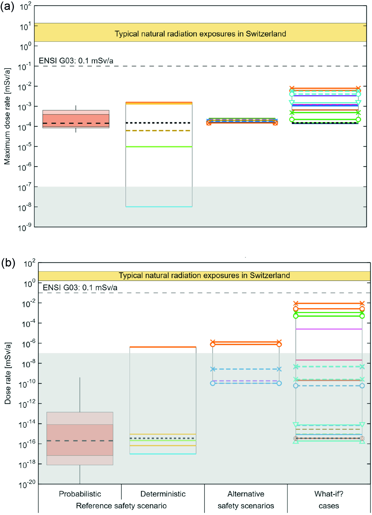
Fig. ‎8‑14:Summary showing the maximum dose rates over 10⁶ years for the aqueous phase transport of all radionuclides and (a) for two-phase transport of ¹⁴C (b)

The reference safety scenario (probabilistic and deterministic calculation cases), calculation cases for the alternative safety scenarios and “what-if?” cases (except the “what-if?” case of excavation) are shown.

The boxplots show the statistical measures of median (dashed horizontal line), 95/5 and 84/16 percentiles (light and dark shades of red) and the full extent of the spread between minimum and maximum (thin vertical line); individual deterministic calculation cases are shown with coloured solid or dashed lines and markers which correspond to the calculation cases in Sections 7.1.5 and 7.2.5 of NTB 24-18 (Nagra 2024p).

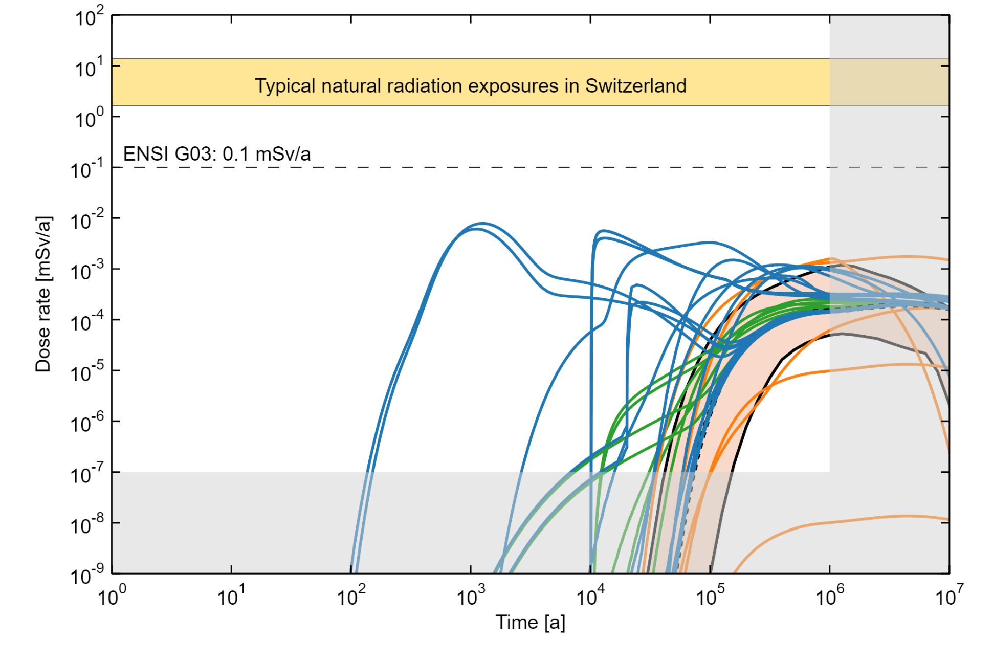
Fig. ‎8‑15:Summary showing dose rates for all the calculation cases for which the dose protection criterion is relevant

The reference case in dashed black, the reference scenario in orange, the alternative safety scenarios in green and the “what-if?” cases in blue lines. The orange surface illustrates the minimum and the maximum of the probabilistic simulations