The embedding of the analysis of radiological consequences in the general safety assessment workflow (see Chapter 4 and Section 5.4 in NTB 24-19,Nagra 2024t) is illustrated in Fig. ‎8‑1. The starting point for the radiological consequence analysis is the set of calculation cases that has been defined in the safety scenario development as requiring quantitative evaluation, as discussed and illustrated in Chapter 7.

Each calculation case is then conceptualised in more detail. Numerical models are developed and parametrised, resulting in a set of calculations to be performed with input parameters for each of them. Care is taken that model abstractions are consistent with those made in PA and that related model uncertainty is bound and understood (see e.g., NAB 24-25, Nagra 2024k and Appendix A and E of NTB 24-18, Nagra 2024p).

The numerical models are composed of near- and far-field components to compute radionuclide release, retention and transport through the engineered barriers and the geosphere (i.e., the Opalinus Clay and the CRZ) and a biosphere model that converts release rates from the geosphere to the biosphere into annual effective doses (Fig. ‎8‑2).

In the near field, the focus is on the release (e.g., degradation and release rates, solubility) and retention (e.g., sorption) of radionuclides. The radionuclide source term is based on the expected inventory as described in Section 5.3.1. Due to the excellent retention properties of the repository barrier system, particularly the CRZ, only a small fraction of the radionuclides needs to be considered when calculating dose rates. These are determined using a screening process, which is based on a highly conservative and simplified transport model and, for the probabilistic calculations, in a second step based on the results of the deterministic calculations. Refer to Section 5.4.1. in NTB 24-19 (Nagra 2024t) for details.

For radiological consequence analysis, the stratigraphic units (host rock and confining units) are considered based on the abstraction shown in Fig. 7‑2 in Section 7.2.2. The geological units are considered as individual transport media in the numerical modelling, whereby some further abstractions are made, such as merging Calcareous Lias CL and Argillaceous Keuper AK3 to a unit KEU. The Keuper aquifer is part of the KAL unit in the numerical abstractions.

For the migration of radionuclides to the boundary of the CRZ, two pathways are considered:

• radionuclide migration in the aqueous phase, in which radionuclides are released to porewater that contacts the waste packages and are subsequently transported by aqueous diffusion and, where there is porewater flow, by advection, and

• radionuclide migration of ¹⁴C in both the liquid and gaseous phase¹⁸, in which ¹⁴C in the form of methane mixes with, and is transported by, other repository-generated gas (hydrogen).

The near-field and geosphere conceptualisations and models for the two pathways differ as follows¹⁹:

• For the aqueous phase calculations, the near field includes either an individual SF or RP-HLW disposal canister, together with its surrounding bentonite buffer, or an individual L/ILW emplacement cavern. The HLW and its surrounding near-field barriers are represented using radially symmetric geometries, while a 2D symmetric representation of the LK90 disposal cavern as described in NAB 23‑01 (Nagra 2023a) is used for the L/ILW near field. The near-field radionuclide release rates from SF and from RP-HLW are computed using the STMAN code (Robinson 2022). Releases from L/ILW are computed with the VPAC code. The main model output providing a source term for geosphere modelling is the total (positive) radial radionuclide flux across the emplacement drift or cavern into the surrounding rock. The geosphere retention and transport model is imple­mented in the PICNIC-TD code (Robinson & Chittenden 2022). The geosphere is modelled as a network of one-dimensional transport paths (called legs), which may represent porous media or discrete features such as fractures, cracks, or channels. Flow and transport parameter values, such as diffusion coefficient, sorption coefficient, and hydraulic con­ductivity, are assigned to each leg and are assumed to be invariant in time and space within an individual leg. The radionuclide flux from different exfiltration points from the leg structure is captured and summed together to obtain the release rate from the geosphere into the biosphere. 

• For the two-phase flow calculations, a 3D model combining both the near field and the geosphere is used. The implementation is based on the TOUGH3 code with its equation-of-state EOS75R module²⁰. It simulates two-phase flow of a gas phase and an aqueous phase and advective- diffusive transport of ¹⁴C as methane, with fully implicit thermo-hydro-mechanical coupling between primary variables (i.e., the state variables of pressure, gas saturation, temperature, mass fractions) and secondary variables (porosity, fluid density, fluid viscosity, capillary pressure) (Jung et al. 2018, Zhang et al. in prep.). In order to account for the different needs of dimen­sionality and discretisation in the near field and geosphere, a so-called “macro-element” approach is adopted, by which the number of the numerical elements is significantly reduced by simplifying the similar and (quasi) symmetrically positioned repository structures along with the surrounding rock to representative macro-elements. ¹⁴C fluxes from the model boundary are captured and summed together to obtain the release rate from the geosphere into the biosphere.

The biosphere model serves to convert radionuclide fluxes to an effective dose by providing so-called biosphere dose conversion factors (BDCFs). These BDCFs are derived from modelling of radionuclide transfer and accumulation processes in the surface environment and of radionuclide pathways leading to the exposure of humans to radioactivity. The biosphere modelling is carried out using a compartment modelling framework and is implemented with the SwiBAC code. For details of the biosphere modelling approach, see NAB 24-06 (Nagra 2024n). The biosphere model is identical for most calculation cases (use of reference biosphere), albeit for the reference safety scenario four different biosphere situations are considered, leading to four separate calculation cases (reference calculation case and three additional calculation cases, as shown in Fig. ‎7‑3). Only the “what-if?” case “excavation of the repository by erosive processes” and some future human action safety scenarios require adaptations of the biosphere model due to potential radionuclide sources directly in the surface environment (for details see NAB 24-08, Nagra 2024q and NAB 24-09, Nagra 2024r).

Note that in general, conservatively, radionuclide fluxes out of the CRZ are directly multiplied by the BDCFs. This corresponds to neglecting the transport time in between the boundary of the CRZ and the biosphere near-surface aquifer, that is, not taking credit for radioactive decay or for dispersion and dilution during this transport. This is illustrated in the scenario figures with the blue dashed lines (e.g., Fig. ‎7‑3).

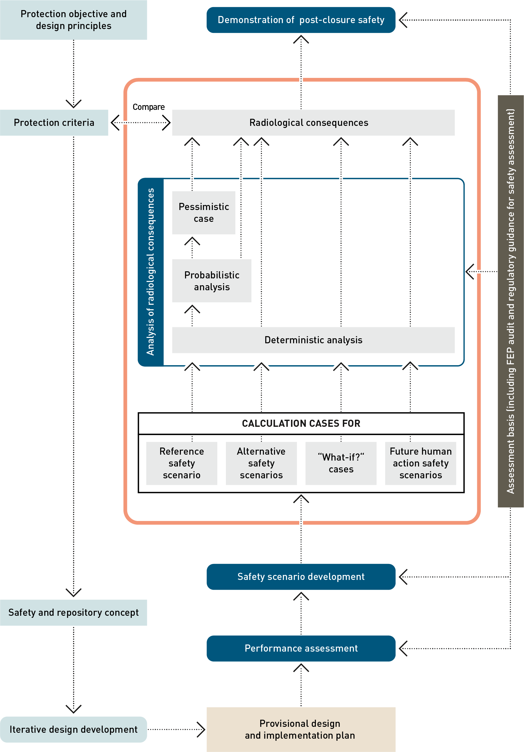
Fig. ‎8‑1:Workflow for the post-closure safety case, highlighting, in the orange box, the main elements of the analysis of radiological consequences

When parametrising the models used in calculations, care is taken to distinguish between realistic (best estimate) values, conservative or pessimistic assumptions, and stylised approaches (see also Section 4.4). In general, when there is quantified uncertainty in the properties of repository features, rates of processes and other model parameters, realistic values and, for the probabilistic calculation case, realistic parameter bandwidths, are assumed. Other uncertainties are generally handled using conservative assumptions. Parameter assumptions and details of the treatment of parameter uncertainty can be found in Appendix C in NTB 24-18 (Nagra 2024p). Stylised assumptions are made where appropriate. They are used in the context of the biosphere modelling, the “what-if?” case of “excavation of the repository by erosive processes” and future human actions safety scenarios. Further, the assumption is made that the different biospheres (e.g., constant climatic conditions) are maintained throughout the time period for assessment.

Once the models and parametrisations are defined, simulations are performed and the results are grouped in the electronic input data and results application (EDR, Nagra 2024p) such that each result can be linked to its input parameters and model chain. Finally, the results are compared with the regulatory protection criteria and the safety margins are evaluated. For this, dose rates as a function of time and the maximum dose rate over the time period for assessment are analysed and compared. For the calculation cases linked to the “what-if?” case of “excavation of the repository by erosive processes”, the risk is also evaluated and compared with the regulatory risk criterion for these calculation cases.

Organic ¹⁴C is considered as methane in both the aqueous phase calculations and in the two-phase flow calculations. Because the entire organic ¹⁴C inventory is considered separately in both calculations, the results are also presented separately as alternative model assumptions, i.e., one in which all methane is assumed to be fully dissolved despite its volatility and the low solubility of methane gas and one in which methane is partitioned between the dissolved and gaseous phases. In fact, summing both results would correspond to counting the organic ¹⁴C inventory twice. A further reason for presenting the results separately is that otherwise the distinct characteristics of the two-phase flow results would be barely visible, since the absolute values of dose rate contributions for these cases are small when compared with the aqueous phase contributions.

Note that, in the graphical representation of the radiological dose calculations shown in the following sections, the grey-shaded areas indicate two aspects:

• Dose rate: Many of the calculations presented in this chapter show very low dose rates. A dose of 10^-7 mSv/a to an individual corresponds to an extremely low overall fatal risk coefficient for the exposed person of 5 × 10^-12 per year²¹. This is reflected in the graphical presentation of such results, where grey shading is used below 10^-7 mSv/a to emphasise that such results have no radiological significance.

• Extended time period: Shading is also used in graphs of dose-rate evolution, where results are presented beyond the time period for assessment of one million years, again to illustrate the behaviour of the models representing the disposal system, as well as to ensure that maximum dose rates are captured.

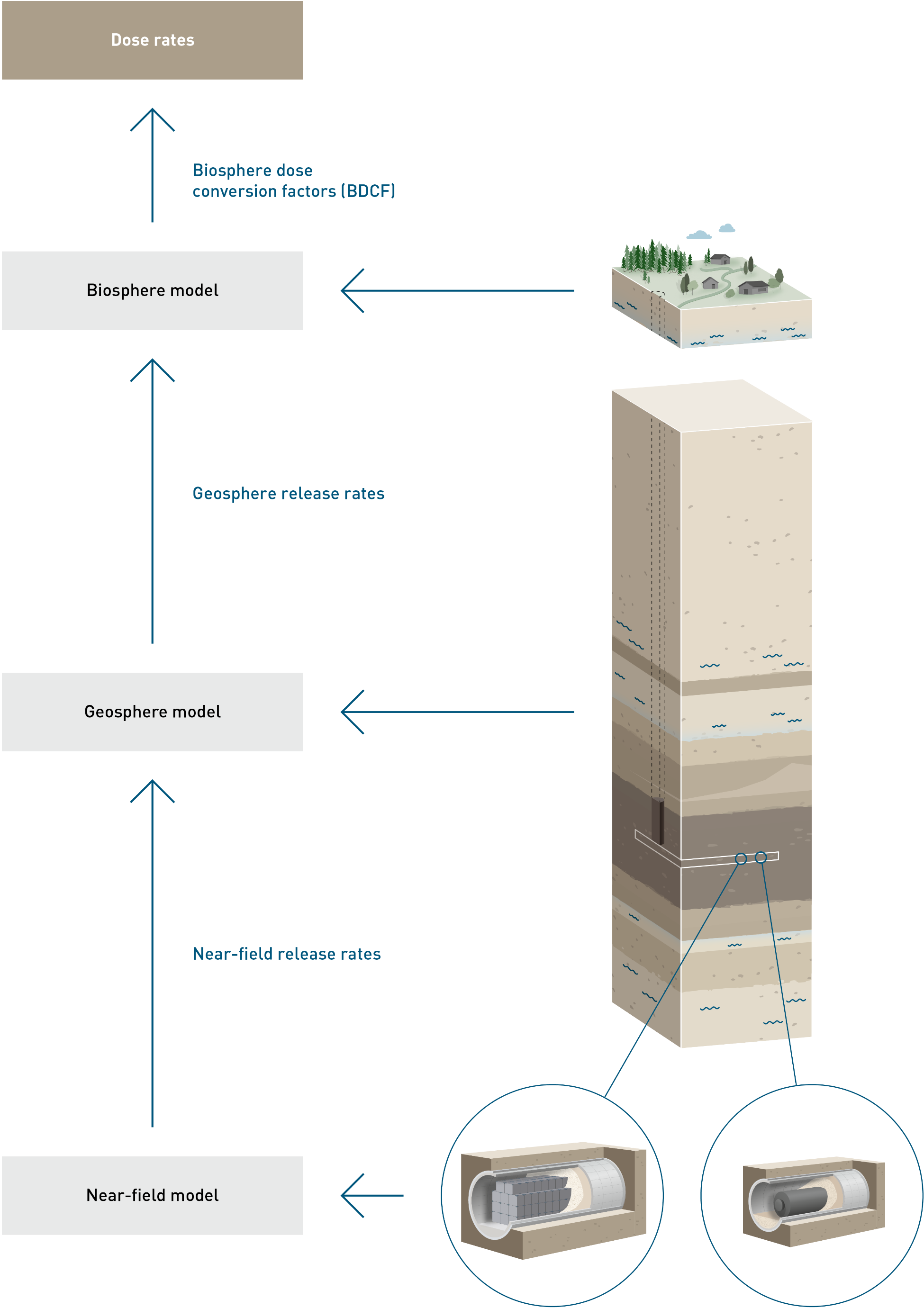
Fig. ‎8‑2:Workflow for the computation of radiological consequences for an individual calculation