
The three-dimensional steady state numerical groundwater flow model (extract of the 3D model shown on Fig. 4‑97) aims to test the consistency of the hydrogeological dataset and provide insights into the groundwater flow systems. It is also a tool to investigate the impact of different conceptualisations, for example with respect to the properties of the hydrogeological units and of the regional faults.
The focus of Sections 4.5.4.2 to 4.5.4.5 is on the identification of the recharge and discharge areas of the main aquifers. These will also feed into the interpretation of the hydrogeochemical data of the groundwater samples to develop a consistent understanding (Section 4.5.6). Note that the hydrogeochemical dataset may also include information on transient processes (e.g. old seawater components) – in contrast to the steady state groundwater flow model.
Technical details on the model are provided by Nagra (2024n). The model extent and the boundary conditions were defined based on available data and earlier modelling results (e.g. Gmünder et al. 2014). The modelling procedure included a sensitivity analysis of the boundary conditions to investigate their impact on the groundwater flow field. The outcome of this analysis led to the selection of a base-case model for further calibration. The calibration was carried out using the PEST algorithm (Doherty 2004) focusing on the hydraulic parameters of the Malm, Hauptrogenstein, Keuper, and Muschelkalk aquifers (Nagra 2024n). The hydraulic properties of the faults were related to the hydraulic properties of the hosting units using multiplicative factors. The latter were adjusted during the final phase of the calibration to further enhance the quality of the fit.
The base-case model includes a no flow boundary condition at the southern limit of the model reflecting the low hydraulic conductivities of the aquifers expected at several kilometres depth. The importance of this choice needs to be put into perspective. Indeed, the sensitivity analysis showed that the hydraulic conditions assigned to the southern boundary have no significant impact on the northern part of the model where the siting regions are located.
The recharge and discharge areas of the aquifers are visualised using backward and forward particle tracking (Fig. 4‑98, Fig. 4‑100, Fig. 4‑101, Fig. 4‑102). These were calculated by post-processing the model results using the simulated groundwater velocity field and generic porosities. The calculation of the particle paths was stopped after an arbitrarily selected time frame of 5 million years. Note that this is not intended to serve as a long-term prediction (steady state model).
Particles were released in the middle of the aquifer horizons above and below the Opalinus Clay in the perimeter of the siting regions. While the released particles usually travel within the bounds of the thick aquifers during the considered time frame, particles released in thin aquifer layers may be trapped in the adjacent aquitards (Nagra 2024n).
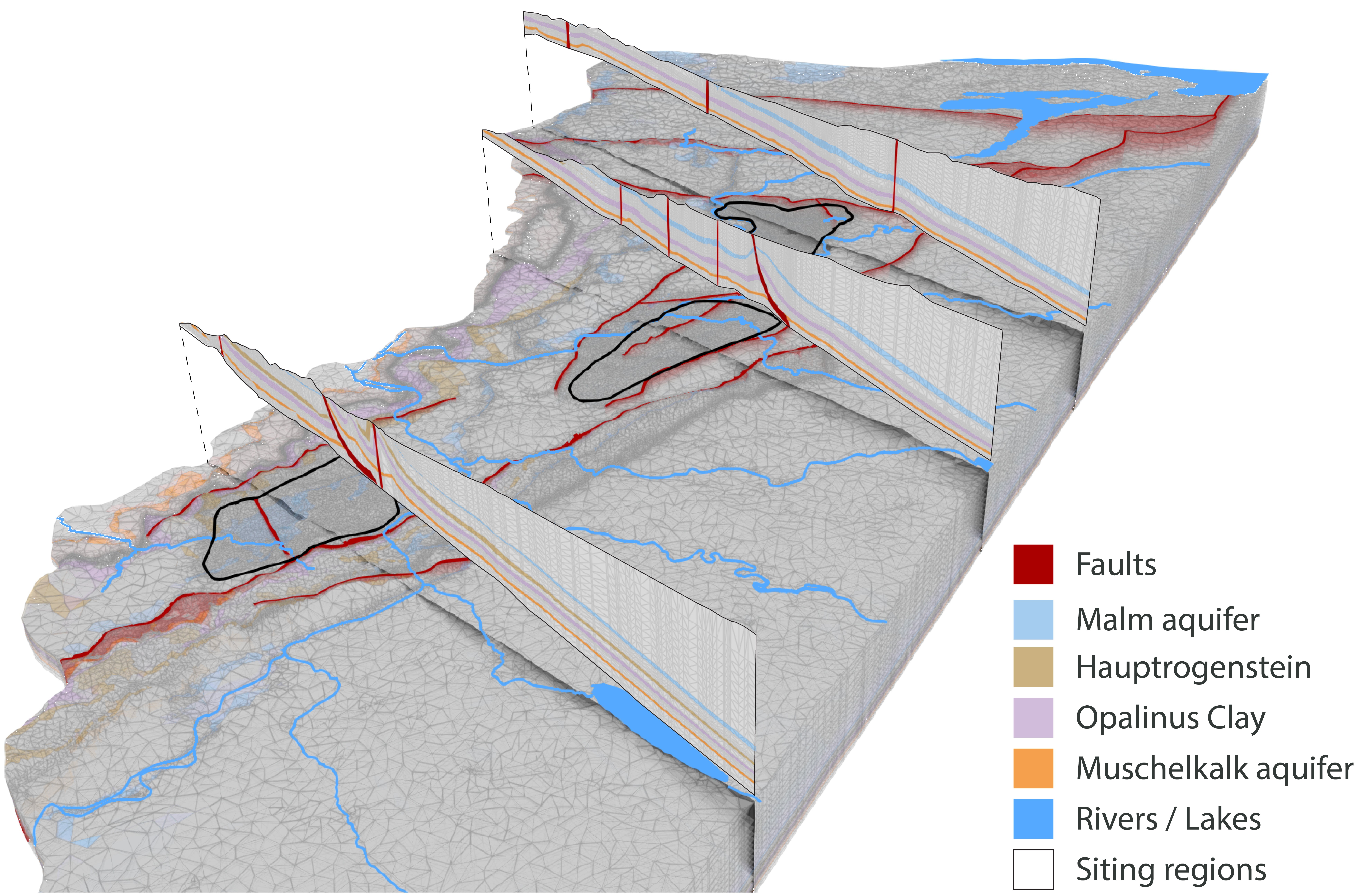
Fig. 4‑97:3D view of the northeastern part of the hydrogeological model, with respective cross-sections showing the main regional aquifers, together with the Opalinus Clay
Model is vertically exaggerated 2×, cross-sections are exaggerated 3×. The Malm aquifer (top of the «Felsenkalke» + «Massenkalk» to the base of the Villigen Formation), Hauptrogenstein aquifer, Opalinus Clay and Muschelkalk aquifer (Schinznach Formation), as well as a simplified regional fault pattern are displayed.