To provide a continuous description of the 3D stress state in the siting regions, geomechanical-numerical models are set up that use point-wise stress magnitude measurements for the model calibration. These models, hereafter "stress models", integrate all geomechanically relevant rock properties of the drilled formations and structural elements. The lateral extent of these stress models is depicted in Fig. 4‑76 and further technical details can be found in Nagra (2024o).

Given that the stiffness distribution, i.e. Young’s Modulus E, exerts a key control on the stress field, the stress models account for stiffness variability. An example of modelling input and results is shown in Fig. 4‑81, with the range of stiffness values on 95% probability (i.e. stiffness value within this range) on the right. The result is a bandwidth of the horizontal stress magnitudes rather than a single line indicating the best fit to the stress magnitude data used as model calibration points. Using this stiffness variation for sensitivity analyses in stress model runs, Fig. 4‑81 shows the resulting 95% probability of stresses that should be expected. This 95% probability band should contain the stress measurements of S_hmin and the derived S_Hmax values, as they also reflect the stiffness variability within the formations. Indeed, except for a few outliers that sampled the formation outside the 95% probability range, most data points are covered by the derived stress band.

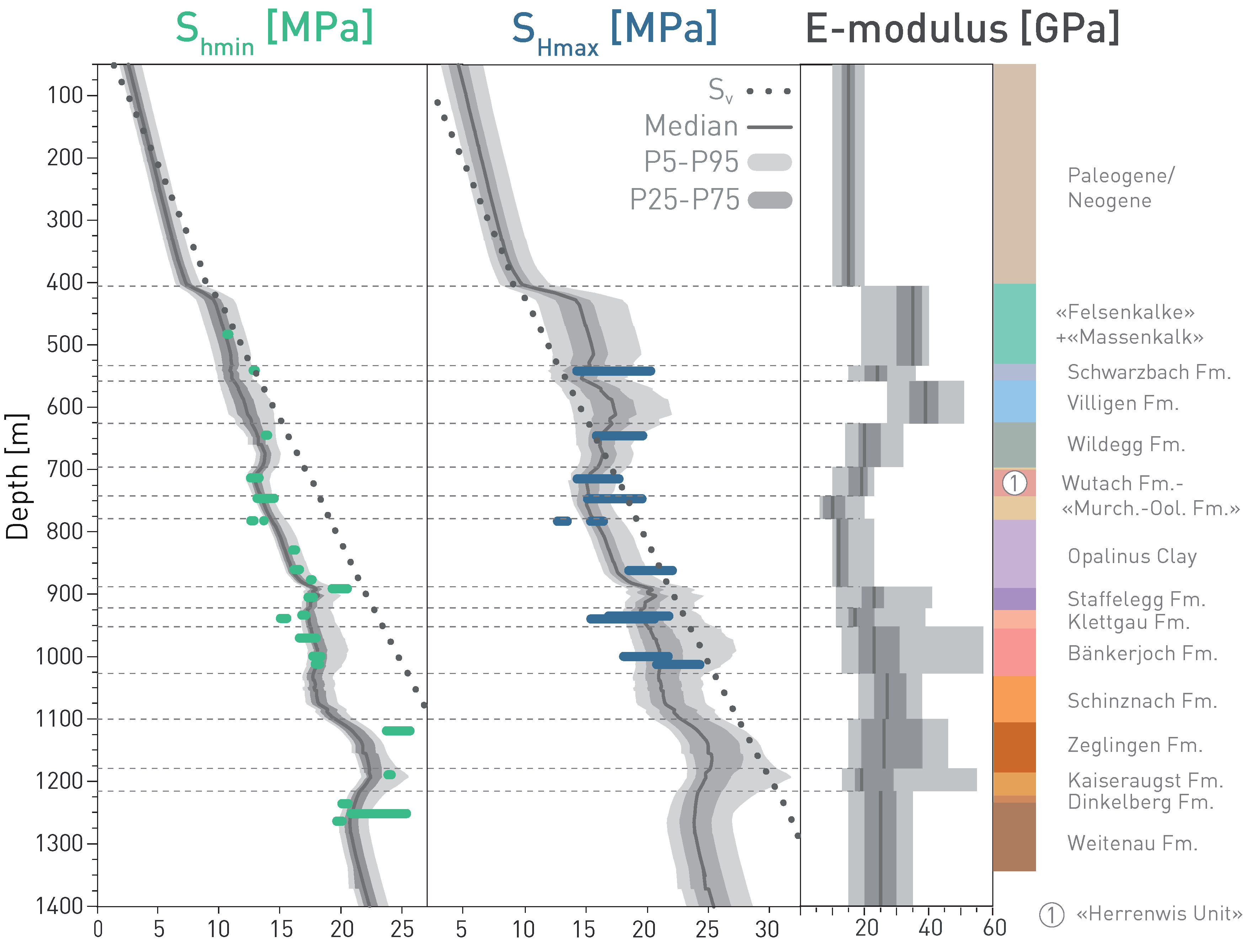
Fig. 4‑81:Stress magnitude data from MHF/SR tests and modelled stress bandwidth

Green and blue bars represent bandwidths of S_hmin and S_Hmax magnitudes from MHF and SR test results from the STA3 borehole. The dotted line depicts S_v. Dark and light grey bands represent the P25 to P75 and P5 to P95 percentile, respectively, and the dark line in the centre represents the P50 value for both, Young’s Modulus E on the right, and the track of the S_hmin and S_Hmax from the stress models.

Stress models were also used to explore the effect of faults on the stress field. It can be shown that this effect is relatively small and is not present a short distance away from the faults (Nagra 2024o, Reiter et al. 2024).

The model results also provide the bandwidth of the stress regime in all formations grouped by site as displayed in Fig. 4‑82. For site comparison, stress values were extracted from the site-specific stress models along a vertical trajectory into the approximate location of the current repository project. The stress regime is expressed using the continuous regime stress ratio (RSR) value (Simpson 1997). As discussed above for the MHF field data only, the stress model runs suggest a normal faulting stress regime for the Opalinus Clay, especially for the NL siting region. For ZNO and especially JO, the dominant stress regime transitions from normal faulting to strike- slip faulting because of the progressively shallower position of the Opalinus Clay. This trend to a higher lateral stress relative to the vertical stress is particularly manifested in the formations above the Opalinus Clay and can reach thrust faulting stress regime conditions (S_Hmax > S_hmin > S_v) in the Malm.

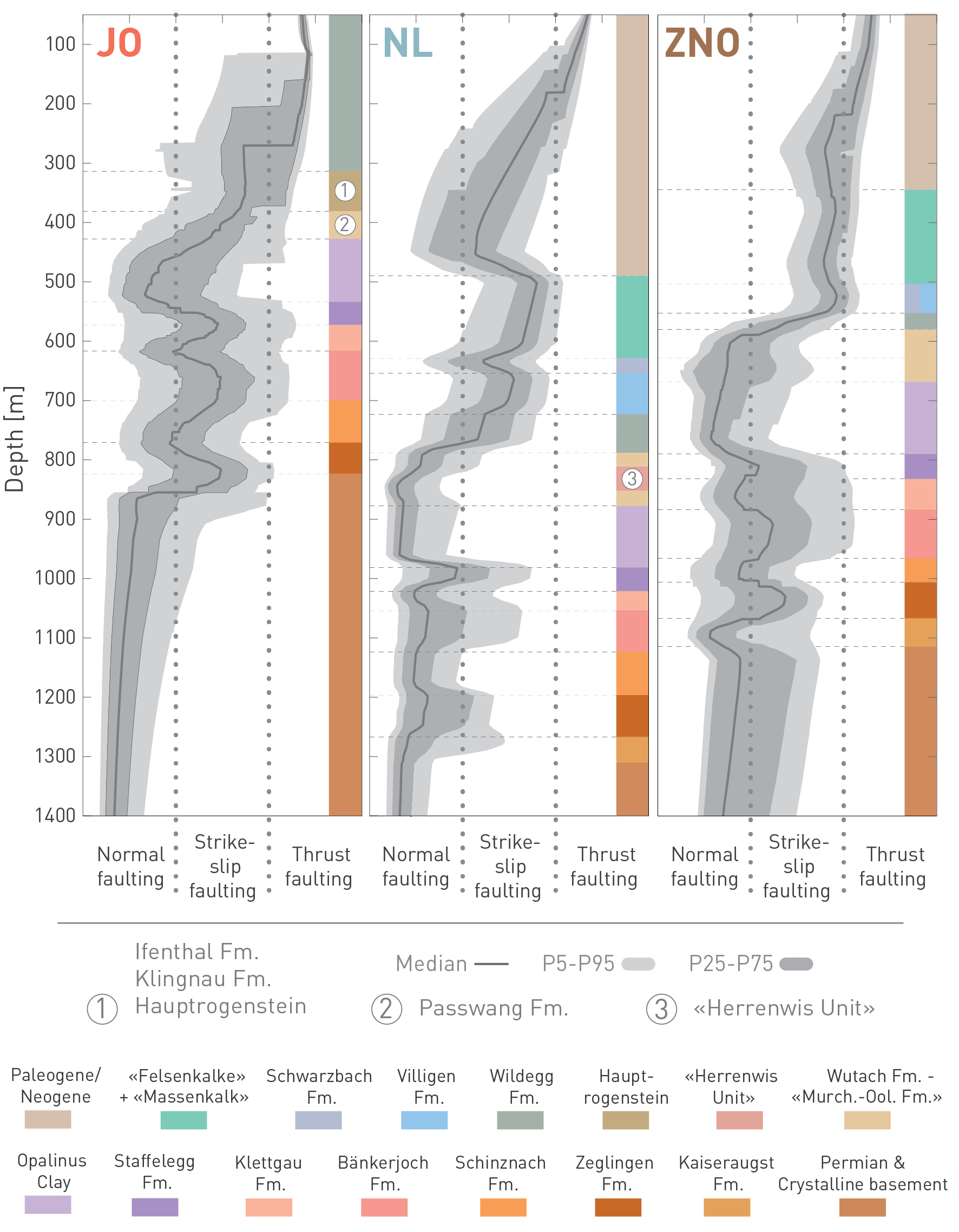
Fig. 4‑82:Comparison of stress regimes within the rock formations across the different siting regions

Values are extracted from stress model runs at a vertical trajectory into the approximate location of the high-level waste section of the current repository project in each site. To assign continuous values of stress regime (x-axis) the classification according to the regime stress ratio is used (details can be found in Nagra 2024o).